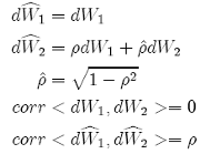
We begin by writing down the usual Geometric Brownian Motion SDE where the volatility σ is written as the square root of a variance ν and is assumed to follow its own SDE:

(15)

where (r − D) is the deterministic instantaneous drift of stock price returns, κ is the mean-reverting speed, θ is the long-run mean, λ is the market price of risk function, ξ is the volatility of volatility, and dW1 and dW2 are two Wiener processes (Brownian motion) with correlation coefficient ρ. We use γ to generalize {15}. The six parameters κ, θ, λ, ξ, γ and ρ are assumed to be constant.

If one wishes to use a Monte Carlo scheme to calculate risk-neutral expectations, we need to find an approximation or discretization of {15}.

Euler and Milstein Scheme for 1D

Using the definition in {9} and {10}, the strong stochastic Taylor approximation of order 0.5 for the {SDE-15}, usually called the 1D Euler scheme (or simply Euler scheme), has the following form:

(16)

and the strong stochastic Taylor approximation of order 1.0 for the {SDE- 15}, called the 1D Milstein scheme, is:

(17)

where: {(∆W1,t)² − ∆t} is called the Milstein correction.

Euler and Milstein Scheme for 2D

Using X1 = S, and X2 = ν, the {SDE-15} can be transformed to a vector with independent noise sources:

(18)

where:

The strong stochastic approximation of order 0.5 for the 2D vector {SDE- 18}, called 2D Euler scheme, remains the same as the Euler scheme for one dimension {SDE-16}. However, after some calculations shown in Appendix 2, the strong stochastic Taylor approximation of order 1.0 for the 2D vector {SDE-18}, called 2D Milstein scheme, is:

(19)

or for Heston model (γ = 1/2):

(20)

where:

(21)

The derivation of the {SDE-19} is explained in more detail in Appendix 2 and, in the next section, is explained how we can approximate the double integral {21}. Simulations, comparisons and conclusions are also given in the end of the chapter.

Prof. Klaus Schmitz

Next: General 2D Milstein scheme for stochastic volatility models

Summary: Index