Option smiles can result either from heterogeneous beliefs, as I have been arguing, or heterogeneous risk tolerance as Benninga-Mayshar (2000) argue.^[43] Empirically, there is evidence of significant heterogeneity in respect to both beliefs and risk tolerance. Is there a compelling reason to structure models that embody both sources of heterogeneity? Is it possible, and plausible, that effects stemming from heterogeneous beliefs could masquerade as effects stemming only from risk tolerance? In other words, could we pretend that investors always hold homogeneous beliefs that are correct, and explain smile effects by appeal to heteroge-neous risk tolerance alone?

To address the last question, consider the log-kernel at date 0,

where m, Λ, θ_R, and g are functions of x₁. Suppose that the true log-kernel is given by m, but we treat Λ as zero, and ask that heterogeneous risk tolerance explain the structure of the pricing kernel.^[44] In order to do so, seek a risk tolerance function θ_Π(x_t) to satisfy

and solve for θ_Π to obtain:

Equation (29) describes the distortion that results from falsely attributing the impact of heterogeneous beliefs to heterogeneous risk tolerance. The magnitude of the distortion is Λ/ ln(g), that being the wedge between θ_Π and θ_R. In this regard, recall that 1/θ_R(x_t) is a convex combination of the individual traders’ risk tolerances {1/θ_h}, with weights α_h given by (6).

To understand the nature of the wedge between θ_R and θ_Π, consider figure 2c which depicts the graphs of ln(g(x_t)), Λ, and m in one of my examples. Observe that Λ dominates m in the figure. In the example underlying figure 2, θ_R(x_t) = 1 because all traders have logarithmic utility (θ_h = 1). Consider the following question: Given the structure of the
θ_R−function, is it plausible for −θ_Πg(x) to capture the impact of Λ?

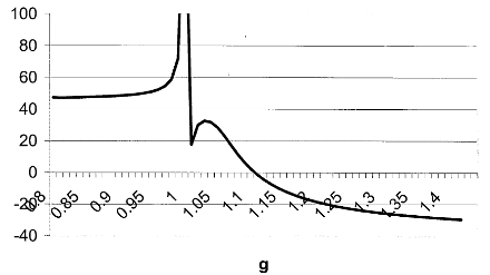
As a general matter, the answer to the previous question is no. To see why, consider figure 9 which displays how the function in (29) varies across g, for the example underlying figure 2. Notice that θ_Π increases from 47 to ∞ as g approaches 1 from the left.45 To the right of the singularity at g = 1, θ_Π rises to a maximum, and then declines, eventually turning negative. What figure 9 illustrates, rather dramatically, is that although it is possible to find a θ_Π−function to capture the impact of sentiment, θ_Π may differ markedly from θ_R = 1. Hence, although it is formally possible to capture the impact of nonzero sentiment through heterogeneous risk tolerance, it is not particularly meaningful, in that θ_Π does not capture the underlying risk tolerances of the individual traders.

Benninga and Mayshar explain that heterogeneous risk tolerance can be a cause of option smiles. Consider how this effect is reflected within the characteristics of their representative trader. I suggest that the key characteristic involves the variation in the function θ_R over x_t. By way of contrast, when traders share the risk tolerance parameter, as in my example discussed above, then θ_R(x_t) = θ_h and so is constant across x_t. However, when there is heterogeneity in risk tolerance, then θ_R(x_t) can vary across x_t, and this is the source for smile effects induced by heterogeneous risk tolerance.

It is important to understand the degree to which the Benninga-Mayshar restriction limits the variation of θ_R across x_t for fixed t. In order to discuss this issue, consider another example where traders’ risk tolerance parameters lie between 0.2 and 1.46 In this example, it turns out that for fixed t, θ_R varies from 0.48 to 0.52, as consumption growth rate varies from 0.95 to 1.06.

The source of variation in θ_R stems from the manner in which α_h(x_t) varies across x_t as we form the convex combination

to obtain 1/θ_R(x_t). In the heterogeneous risk tolerance example described above, one of the corresponding α_h−functions might vary, say, from 0.23 to 0.26. Further insight into the degree to which α_h varies can be obtained by combining equations (5) and (6). Doing so implies that α_h and θ_R jointly satisfy:

Notice that (30) implies that the greatest variation in α_h across x_t occurs for those traders who possess the most extreme values of θ_h.

This degree of variation in θ_R is quite moderate, and contrasts sharply with the degree of variation exhibited by θ_Π. In contrast to the θ_Π depicted in figure 9, the degree of variation in θ_R across states tends to be small. Because 1/θ_R is a convex combination of 1/θ_h− parameters, it lies between the minimum and maximum values of 1/θ_h in the trading population. Notice that θ_Π moves well outside this range. Indeed (29) implies that when Λ is nonzero, θ_Π must lie outside this range for g close to 1. Moreover, θ_R is defined independently of traders’ beliefs. Therefore, as a general matter, it is not possible to attribute the impact of heterogeneous beliefs to heterogeneous risk tolerance in a reasonable manner.

In a related vein, I note that because of wealth shifts stemming from trading, the conditional one-period function θ_R− may vary over time. For instance, suppose that wealth is initially concentrated in the hands of the trader with the lowest risk tolerance parameter,
but over time loses his wealth to the trader with the highest risk tolerance. Then over time, the conditional θ_R−function will move from the region around the lowest risk tolerance parameter to the highest. Notice that this intertemporal instability in conditional θ_R is different from the stability of the θ_R−function for fixed t.

There is an implicit premise in the paper, namely that at the level of the individual trader risk tolerance is a permanent characteristic. However, no such premise applies to beliefs. Beliefs can be quite volatile at the level of the individual trader, and therefore sentiment too can be volatile.

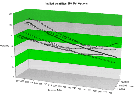
Consider figure 10, which is taken from Shefrin (1999). It depicts the time varying nature of implied volatilities for S&P 500 index put options in the period November-December 1996. Notice the dramatic change in the strength of the smile effect over this period. Given the nature of α_h, I suggest that it is implausible to explain this change on the basis of time variation in θ_R, induced by variations in the α_h−functions.

The comments in the preceding paragraph are related to those I made in section 5, as regards the volatility of the pricing kernel. As I mentioned there, Campbell (2000) points out the volatility of the SDF appears to be puzzling high for a variable that is bounded below by zero and whose mean is unity. His observation is based on the fact that the coefficient of variation of the SDF is bounded from below by the maximum Sharpe ratio across securities. However, the SDF that Campbell discusses implicitly treats sentiment as zero.

To be sure, heterogeneity in risk tolerance can produce smile effects in option prices. A similar remark applies to stochastic volatility in fundamental variables. I would call the associated smile patterns efficient, in that they arise in models where prices are objective. However, the focal point of this paper concerns the impact of nonzero sentiment stemming from heterogeneous beliefs. The latter also produces smile effects, but I argue that those smile effects reflect inefficiencies in pricing. I call them “inefficient smiles.” Heterogeneity in risk tolerance may cause smile effects, but those effects are manifestations of efficiency. Heterogeneity in risk tolerance gives rise to efficient wrinkles, not the inefficient kernel-smiles (as depicted in figure 2c) nor the mean-variance frowns (as depicted in figure 8b). Of course, there is no reason to exclude one source of heterogeneity at the expense of the other. The theory in this paper allows for both to be accommodated.

Prof. Hersh Shefrin

Next: Conclusion and Future Directions

Summary: Index