This appendix contains proofs of theorems 1, 5, 7, and 8. Theorem 2 is essentially proved in the body of the paper. Theorem 3 follows directly from equation (5). Theorem 4 is proved in the body of the paper. The proof of theorem 6 is similar to the proof of theorem 5, and relies on equation (5). Additional commentary pertains to theorem 2 in Shefrin-Statman (1994), and the uniqueness of state prices.

Proof of theorem 1

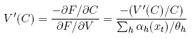
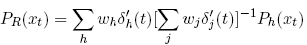
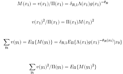
The plan of the proof is to derive expressions for P_R, θ_R, and δ_R, by equating two different expressions for g(x_t). The first expression for g(x_t) stems from the equilibrium condition

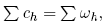
where ch is given by (4). The second expression for g(xt) stems from (5) which expresses equilibrium prices v in terms of g(x_t) and the representative trader’s parameters P_R, θ_R, and δ_R.

I begin the proof by defining

and

which is equivalent to the expression for (x_t) that appears just before the statement of Theorem 1. Next turn to the two expressions for g(x_t). The first uses (4) to compute the equilibrium value of g(x_t). By definition,

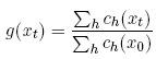
and substituting for c_h from (4), obtain

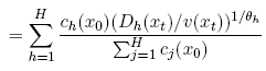
which, using the definition of Υ_h, yields

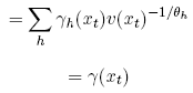
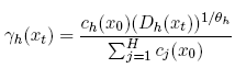
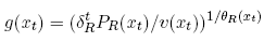
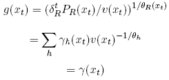
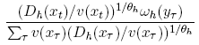
by the definition of Υ The second expression for g(x_t) is obtained by inverting equation (5). Doing so yields:

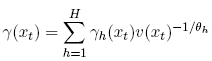
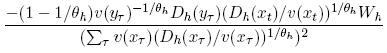
Now equate the two expressions for g(x_t) to obtain:

In the remainder of the proof, I use the last set of equations to establish the expressions for P_R, δ_R, and θ_R that appear in the statement of theorem 1. Notice that the preceding equation, equating the two terms for g(x_t), implies that:

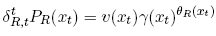
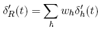
Hence, the preceding equation defines δ^t_R,t P_r(x_t) in terms of θ_R. Define δ^t_R,t as the following sum, for fixed t:

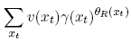
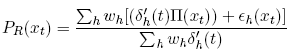
Then define P_r(x_t) as the ratio

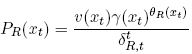
In view of the normalization implicit in the last equation,

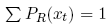
for each t. Nonnegativity of P_r follows from the fact that all variables involved in the construction are nonnegative. With δ^t_R,t and P_r(x_t) defined in terms of θ_R, it remains to specify θ_R. In this respect, let θ_R be (8). Notice that (8) is a function of Π, and is derived from Benninga- Mayshar (1993). In particular, (8) is not dependent on P_r or θ_R. Hence there is no issue of simultaneity in determining δ^t_R,t , P_r(x_t), and θ_R.

The preceding argument establishes the first part of the theorem. In order to establish the nonuniqueness claim, observe that we are free to specify the function θ_R. Instead of choosing (8), the Benniga-Mayshar expression, we could also have set θ_R(x_t) equal to an arbitrary constant for all xt, and solved for P_r and θ_R, again, as functions of θ_R. Equation (11) follows from (5). For sake of completeness, I sketch the proof provided by Benninga and Mayshar (1993) characterizing θ_R. Note that (4) and

imply that

for all x_t. Based on (4), the equilibrium condition

0, and the kernel variable V = v/Π, Benninga-Mayshar define the implicit function

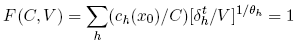
They note that by the principle of expected utility maximization, the representative trader’s marginal utility at C will be proportional to V . In turn, this implies that θ_R, the Arrow- Pratt coefficient of relative risk aversion can be defined locally by −CV 0(C)/V (C). By
computing ðF/ðC and ðF/ðV , they observe that

which, taken together with the local Arrow-Pratt measure, completes their proof. Case of log-utility: beliefs of representative trader and objective prices Consider the nature of theorem 1 in the special case when θ_h= 1 for all h, this being the case of log-utility. Shefrin and Statman (1994) use (3) to establish that the representative trader’s beliefs are given by the weighted sum:

and the representative trader’s normalized discount factor is:

These expressions are obtained by using (3) to equate ∑_hC_h(x_t) and C_r(x_t) to obtain the expression for P_r, and equating ∑_h,xt C_h(x_t) and ∑_xt C_r(x_t) for fixed t to obtain δ¹_r(t). By definition of ε and the preceding expression for P_r, obtain

so that

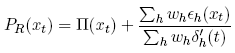
It follows that in order for the efficiency condition P_r(x_t) = Π(x_t) to hold, the sum
∑_h W _hε_h(x_t) must be zero. Define the covariance cov{∑_h W _hε_h(x_t) } by:

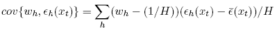
where

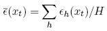
Multiplying out the terms in the covariance, yields the equivalent covariance expression:

for each x_t. Recall that prices are efficient if and only if ∑_h W _hε_h = 0 for all x_t. This is equivalent to

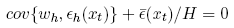
Multiplication of this last expression by PhWh yields the equivalent condition

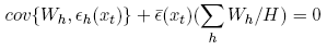
which implies that prices are efficient if and only if the sum of the error-wealth covariance and product of the average error and mean wealth is equal to zero.^[53]

Uniqueness of state prices

Arrow and Hahn (1971) survey conditions under which the equilibrium state price vector v is unique. Their theorem 5, p. 220 establishes uniqueness for the case of homogeneous traders. More generally, their theorem 7, p. 222, establishes that equilibrium state prices are unique if the gross substitute condition holds. The gross substitute condition states that

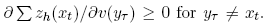
Consider (3), the demand function for an individual trader. In this regard, note that Wh is a dot product of v and ω_h. Differentiation of (3) with respect to v(y_τ) yields an expression that is the sum of two terms. The first term is

and the second term is

Note that the first sum is nonnegative, and when θ_h = 1, the second term is zero. Summation over h leads to

. Computation reveals that the derivative is strictly positive for θ_h ≤ 1, and is therefore positive in an open set of 1.

Proof of theorem 5
From the perspective of x_t−1, η(x_t) is the future value of a contingent x_t real dollar payoff. Given x_t−1, the future value of a contract which delivers a certain dollar at date t must be one dollar. This is why

In other words, the future value of y_t−claims are nonnegative and sum to unity. Hence they constitute a probability distribution. Since they deal with the transition from x_t−1, {η(y_t)} are one-step branch probabilities of a stochastic process.

Under the stochastic process, the probability attached to the occurrence of xt is obtained by multiplying the one-step branch probabilities leading to x_t. To interpret this product, consider the denominator of (20). This term can be matched with the numerator of the x_t−1 one-step branch probability to form

The latter term is simply one plus the single period risk free interest rate i1(x_t−1) that applies on the x_t−1-market. Therefore the probability of the branch leading to x_t is the product of the single period stochastic interest rates and the present value of an x_t-claim: i1(x₀)i1(x₁) ... i1(x_t−1)v(x_t). The product of the single period interest rates defines the cumulative return it c(x_t) to holding the short-term risk-free security, with reinvestment, from date 0 to date t. A call option pays q_z(x_t)−K at date t,

the set of date-event pairs where the option expires in-the-money. The present value of the claims that make up the option payoff is computed using state prices v. But the present value of an x_t−contingent dollar is its future value discounted back by the product of the one-period risk-free rates. The discounted contingent future dollar is simply the ratio of a risk-neutral probability η(x_t) to a compounded interest rate i_c(x_t). Finally, the risk-neutral probability η(x_t) is unconditional. To convert to a distribution conditional on exercise, divide η(x_t) by P_η{A_E|x₀}. Using the conditional expectation in place of the unconditional expectation leads to the appearance of P_η{A_E|x₀} in (21).

Proof of theorem 7

To prove theorem 7, compute the first-order-condition associated with maximizing expected quadratic utility.

(31)

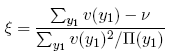
where ξ is the Lagrange multiplier for the optimization and has the form:

(32)

Next observe that

Substitution into (32) completes the proof.

Proof of theorem 8

The proof of this theorem is computational. The one-period return to the market portfolio is the sum of the date 1 dividend and date 1 price, divided by the date 0 price, i.e.

Use (7) to compute the present values two future aggregate consumption stream: the value of the unconditional process under v, and the value of the process, conditional on x₁. The present value of these two streams appear respectively, in the denominator and numerator of (28), with the numerator value divided by v(x₁). This completes the proof.

Prof. Hersh Shefrin

Summary: Index