Certain forms of nonlinear model can be fitted by Generalized Linear Models (glm()). But in the majority of cases we have to approach the nonlinear curve fitting problem as one of nonlinear optimization. R’s nonlinear optimization routines are optim() and nlm(), which take the place of S-Plus’s ms() and nlminb(). We seek the parameter values that minimize some index of lack-of-fit, and nlm() does that by trying out various parameter values iteratively. Unlike linear regression for example, there is no guarantee that the procedure will converge on satisfactory estimates. nlm() requires initial guesses about what parameter values to try, and convergence depends critically upon the quality of the initial guesses.
Least squares
One way to fit a nonlinear model is by minimizing the sum of the squared errors (SSE) or residuals. This method makes sense if the observed errors could have plausibly arisen from a normal distribution. Here is an example from Bates & Watts (1988), page 51. The data are:
> x <- c(0.02, 0.02, 0.06, 0.06, 0.11, 0.11, 0.22, 0.22, 0.56, 0.56, 1.10, 1.10)
> y <- c(76, 47, 97, 107, 123, 139, 159, 152, 191, 201, 207, 200)
The model to be fitted is:
> fn <- function(p) sum((y - (p[1] * x)/(p[2] + x))^2)
In order to do the fit we need initial estimates of the parameters. One way to find sensible starting values is to plot the data, guess some parameter values, and superimpose the model curve using those values.
> plot(x, y)
> xfit <- seq(.02, 1.1, .05)
> yfit <- 200 * xfit/(0.1 + xfit)
> lines(spline(xfit, yfit))
We could do better, but these starting values of 200 and 0.1 seem adequate. Now do the fit:
> out <- nlm(fn, p = c(200, 0.1), hessian = TRUE)
After the fitting, out$minimum is the SSE, and out$estimate are the least squares estimates of the parameters. To obtain the approximate standard errors (SE) of the estimates we do:
> sqrt(diag(2*out$minimum/(length(y) - 2) * solve(out$hessian)))
The 2 in the line above represents the number of parameters. A 95% confidence interval would be the parameter estimate ± 1.96 SE. We can superimpose the least squares fit on a new plot:
> plot(x, y)
> xfit <- seq(.02, 1.1, .05)
> yfit <- 212.68384222 * xfit/(0.06412146 + xfit)
> lines(spline(xfit, yfit))
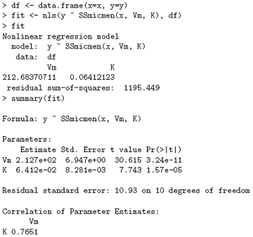
The standard package stats provides much more extensive facilities for fitting non-linear models by least squares. The model we have just fitted is the Michaelis-Menten model, so we can use

Maximum likelihood
Maximum likelihood is a method of nonlinear model fitting that applies even if the errors are not normal. The method finds the parameter values which maximize the log likelihood, or equivalently which minimize the negative log-likelihood. Here is an example from Dobson (1990), pp. 108–111. This example fits a logistic model to dose-response data, which clearly could also be fit by glm(). The data are:
> x <- c(1.6907, 1.7242, 1.7552, 1.7842, 1.8113, 1.8369, 1.8610, 1.8839)
> y <- c( 6, 13, 18, 28, 52, 53, 61, 60)
> n <- c(59, 60, 62, 56, 63, 59, 62, 60)
The negative log-likelihood to minimize is:

We pick sensible starting values and do the fit:
> out <- nlm(fn, p = c(-50,20), hessian = TRUE)
After the fitting, out$minimum is the negative log-likelihood, and out$estimate are the maximum likelihood estimates of the parameters. To obtain the approximate SEs of the estimates we do:
> sqrt(diag(solve(out$hessian)))
A 95% confidence interval would be the parameter estimate ± 1.96 SE.
Some non-standard models
We conclude this chapter with just a brief mention of some of the other facilities available in R for special regression and data analysis problems.
• Mixed models. The user-contributed nlme package provides functions lme() and nlme() for linear and non-linear mixed-effects models, that is linear and non-linear regressions in which some of the coefficients correspond to random effects. These functions make heavy use of formulae to specify the models.
• Local approximating regressions. The loess() function fits a nonparametric regression by using a locally weighted regression. Such regressions are useful for highlighting a trend in messy data or for data reduction to give some insight into a large data set. Function loess is in the standard package stats, together with code for projection pursuit regression.
• Robust regression. There are several functions available for fitting regression models in a way resistant to the influence of extreme outliers in the data. Function lqs in the recommended package MASS provides state-of-art algorithms for highly-resistant fits. Less resistant but statistically more efficient methods are available in packages, for example function rlm in package MASS.
• Additive models. This technique aims to construct a regression function from smooth additive functions of the determining variables, usually one for each determining variable. Functions avas and ace in package acepack and functions bruto and mars in package mda provide some examples of these techniques in user-contributed packages to R. An extension is Generalized Additive Models, implemented in user-contributed packages gam and mgcv.
• Tree-based models. Rather than seek an explicit global linear model for prediction or interpretation, tree-based models seek to bifurcate the data, recursively, at critical points of the determining variables in order to partition the data ultimately into groups that are as homogeneous as possible within, and as heterogeneous as possible between. The results often lead to insights that other data analysis methods tend not to yield. Models are again specified in the ordinary linear model form. The model fitting function is tree(), but many other generic functions such as plot() and text() are well adapted to displaying the results of a tree-based model fit in a graphical way. Tree models are available in R via the user-contributed packages rpart and tree.
Next: Graphical procedures
Summary: Index