The basic function for fitting ordinary multiple models is lm(), and a streamlined version of the call is as follows:

> fitted.model <- lm(formula, data = data.frame)

For example

> fm2 <- lm(y ~ x1 + x2, data = production)

would fit a multiple regression model of y on x1 and x2 (with implicit intercept term). The important (but technically optional) parameter data = production specifies that any variables needed to construct the model should come first from the production data frame. This is the case regardless of whether data frame production has been attached on the search path or not.

Generic functions for extracting model information

The value of lm() is a fitted model object; technically a list of results of class "lm". Information about the fitted model can then be displayed, extracted, plotted and so on by using generic functions that orient themselves to objects of class "lm". These include

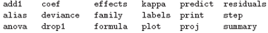
A brief description of the most commonly used ones is given below.

anova(object_1, object_2) Compare a submodel with an outer model and produce an analysis of variance table.

coef(object) Extract the regression coefficient (matrix). Long form: coefficients(object).

deviance(object) Residual sum of squares, weighted if appropriate.

formula(object) Extract the model formula.

plot(object) Produce four plots, showing residuals, fitted values and some diagnostics.

predict(object, newdata=data.frame) The data frame supplied must have variables specified with the same labels as the original. The value is a vector or matrix of predicted values corresponding to the determining variable values in data.frame.

print(object) Print a concise version of the object. Most often used implicitly.

residuals(object) Extract the (matrix of) residuals, weighted as appropriate.Short form: resid(object).

step(object) Select a suitable model by adding or dropping terms and preserving hierarchies. The model with the largest value of AIC (Akaike’s An Information Criterion) discovered in the stepwise search is returned.

summary(object) Print a comprehensive summary of the results of the regression analysis.

Analysis of variance and model comparison

The model fitting function aov(formula, data=data.frame) operates at the simplest level in a very similar way to the function lm(). It should be noted that in addition aov() allows an analysis of models with multiple error strata such as split plot experiments, or balanced incomplete block designs with recovery of inter-block information. The model formula

response ~ mean.formula + Error(strata.formula)

specifies a multi-stratum experiment with error strata defined by the strata.formula. In the simplest case, strata.formula is simply a factor, when it defines a two strata experiment, namely between and within the levels of the factor. For example, with all determining variables factors, a model formula such as that in:

> fm <- aov(yield ~ v + n*p*k + Error(farms/blocks), data=farm.data)

would typically be used to describe an experiment with mean model v + n*p*k and three error strata, namely “between farms”, “within farms, between blocks” and “within blocks”.

ANOVA tables

Note also that the analysis of variance table (or tables) are for a sequence of fitted models. The sums of squares shown are the decrease in the residual sums of squares resulting from an inclusion of that term in the model at that place in the sequence. Hence only for orthogonal experiments will the order of inclusion be inconsequential. For multistratum experiments the procedure is first to project the response onto the error strata, again in sequence, and to fit the mean model to each projection. For further details, see Chambers & Hastie (1992). A more flexible alternative to the default full ANOVA table is to compare two or more models directly using the anova() function.

> anova(fitted.model.1, fitted.model.2, ...)

The display is then an ANOVA table showing the differences between the fitted models when fitted in sequence. The fitted models being compared would usually be an hierarchical sequence, of course. This does not give different information to the default, but rather makes it easier to comprehend and control.

Updating fitted models

The update() function is largely a convenience function that allows a model to be fitted that differs from one previously fitted usually by just a few additional or removed terms. Its form is

> new.model <- update(old.model, new.formula)

In the new.formula the special name consisting of a period, ‘.’, only, can be used to stand for “the corresponding part of the old model formula”. For example,

> fm05 <- lm(y ~ x1 + x2 + x3 + x4 + x5, data = production)

> fm6 <- update(fm05, . ~ . + x6)

> smf6 <- update(fm6, sqrt(.) ~ .)

would fit a five variate multiple regression with variables (presumably) from the data frame production, fit an additional model including a sixth regressor variable, and fit a variant on the model where the response had a square root transform applied. Note especially that if the data= argument is specified on the original call to the model fitting function, this information is passed on through the fitted model object to update() and its allies.

The name ‘.’ can also be used in other contexts, but with slightly different meaning. For example

> fmfull <- lm(y ~ . , data = production)

would fit a model with response y and regressor variables all other variables in the data frame production. Other functions for exploring incremental sequences of models are add1(), drop1() and step(). The names of these give a good clue to their purpose, but for full details see the on-line help.

Generalized linear models

Generalized linear modeling is a development of linear models to accommodate both non-normal response distributions and transformations to linearity in a clean and straightforward way. A generalized linear model may be described in terms of the following sequence of assumptions:

• There is a response, y, of interest and stimulus variables x1, x2, . . . , whose values influence the distribution of the response.

• The stimulus variables influence the distribution of y through a single linear function, only. This linear function is called the linear predictor, and is usually written

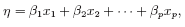
hence xi has no influence on the distribution of y if and only if βi = 0.

• The distribution of y is of the form

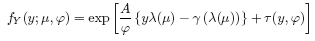
where φ is a scale parameter (possibly known), and is constant for all observations, A represents a prior weight, assumed known but possibly varying with the observations, and µ is the mean of y. So it is assumed that the distribution of y is determined by its mean and possibly a scale parameter as well.

• The mean, µ, is a smooth invertible function of the linear predictor:

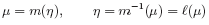
and this inverse function, `(), is called the link function. These assumptions are loose enough to encompass a wide class of models useful in statistical practice, but tight enough to allow the development of a unified methodology of estimation and inference, at least approximately. The reader is referred to any of the current reference works on the subject for full details, such as McCullagh & Nelder (1989) or Dobson (1990).

Next: Families

Summary: Index