Arrays

An array can be considered as a multiply subscripted collection of data entries, for example numeric. R allows simple facilities for creating and handling arrays, and in particular the special case of matrices. A dimension vector is a vector of non-negative integers. If its length is k then the array is k-dimensional, e.g. a matrix is a 2-dimensional array. The dimensions are indexed from one up to the values given in the dimension vector. A vector can be used by R as an array only if it has a dimension vector as its dim attribute. Suppose, for example, z is a vector of 1500 elements. The assignment

> dim(z) <- c(3,5,100)

gives it the dim attribute that allows it to be treated as a 3 by 5 by 100 array. Other functions such as matrix() and array() are available for simpler and more natural looking assignments.

The values in the data vector give the values in the array in the same order as they would occur in FORTRAN, that is “column major order,” with the first subscript moving fastest and the last subscript slowest. For example if the dimension vector for an array, say a, is c(3,4,2) then there are 3 × 4 × 2 = 24 entries in a and the data vector holds them in the order a[1,1,1], a[2,1,1], ..., a[2,4,2], a[3,4,2].

Arrays can be one-dimensional: such arrays are usually treated in the same way as vectors (including when printing), but the exceptions can cause confusion.

Array indexing. Subsections of an array

Individual elements of an array may be referenced by giving the name of the array followed by the subscripts in square brackets, separated by commas. More generally, subsections of an array may be specified by giving a sequence of index vectors in place of subscripts; however if any index position is given an empty index vector, then the full range of that subscript is taken. Continuing the previous example, a[2,,] is a 4×2 array with dimension vector c(4,2) and data vector containing the values

c(a[2,1,1], a[2,2,1], a[2,3,1], a[2,4,1], a[2,1,2], a[2,2,2], a[2,3,2], a[2,4,2])

in that order. a[,,] stands for the entire array, which is the same as omitting the subscripts entirely and using a alone. For any array, say Z, the dimension vector may be referenced explicitly as dim(Z) (on either side of an assignment). Also, if an array name is given with just one subscript or index vector, then the corresponding values of the data vector only are used; in this case the dimension vector is ignored. This is not the case, however, if the single index is not a vector but itself an array, as we next discuss.

Index arrays

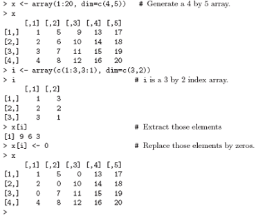
As well as an index vector in any subscript position, an array may be used with a single index array in order either to assign a vector of quantities to an irregular collection of elements in the array, or to extract an irregular collection as a vector. A matrix example makes the process clear. In the case of a doubly indexed array, an index matrix may be given consisting of two columns and as many rows as desired. The entries in the index matrix are the row and column indices for the doubly indexed array. Suppose for example we have a 4 by 5 array X and we wish to do the following:

• Extract elements X[1,3], X[2,2] and X[3,1] as a vector structure, and

• Replace these entries in the array X by zeroes.

In this case we need a 3 by 2 subscript array, as in the following example.

As a less trivial example, suppose we wish to generate an (unreduced) design matrix for a block design defined by factors blocks (b levels) and varieties (v levels). Further suppose there are n plots in the experiment. We could proceed as follows:

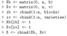
To construct the incidence matrix, N say, we could use

> N <- crossprod(Xb, Xv)

However a simpler direct way of producing this matrix is to use table():

> N <- table(blocks, varieties)

The array() function

As well as giving a vector structure a dim attribute, arrays can be constructed from vectors by the array function, which has the form

> Z <- array(data_vector, dim_vector)

For example, if the vector h contains 24 or fewer, numbers then the command

> Z <- array(h, dim=c(3,4,2))

would use h to set up 3 by 4 by 2 array in Z. If the size of h is exactly 24 the result is the same as

> dim(Z) <- c(3,4,2)

However if h is shorter than 24, its values are recycled from the beginning again to make it up to size 24. As an extreme but common example

> Z <- array(0, c(3,4,2))

makes Z an array of all zeros. At this point dim(Z) stands for the dimension vector c(3,4,2), and Z[1:24] stands for the data vector as it was in h, and Z[] with an empty subscript or Z with no subscript stands for the entire array as an array. Arrays may be used in arithmetic expressions and the result is an array formed by elementby- element operations on the data vector. The dim attributes of operands generally need to be the same, and this becomes the dimension vector of the result. So if A, B and C are all similar arrays, then > D <- 2*A*B + C + 1

makes D a similar array with its data vector being the result of the given element-by-element operations. However the precise rule concerning mixed array and vector calculations has to be considered a little more carefully.

Mixed vector and array arithmetic. The recycling rule

The precise rule affecting element by element mixed calculations with vectors and arrays is somewhat quirky and hard to find in the references. From experience we have found the following to be a reliable guide.

• The expression is scanned from left to right.

• Any short vector operands are extended by recycling their values until they match the size of any other operands.

• As long as short vectors and arrays only are encountered, the arrays must all have the samedim attribute or an error results.

• Any vector operand longer than a matrix or array operand generates an error.

• If array structures are present and no error or coercion to vector has been precipitated, the result is an array structure with the common dim attribute of its array operands.

The outer product of two arrays

An important operation on arrays is the outer product. If a and b are two numeric arrays, their outer product is an array whose dimension vector is obtained by concatenating their two dimension vectors (order is important), and whose data vector is got by forming all possible products of elements of the data vector of a with those of b. The outer product is formed by the special operator %o%:

> ab <- a %o% b

An alternative is

> ab <- outer(a, b, "*")

The multiplication function can be replaced by an arbitrary function of two variables. For example if we wished to evaluate the function f(x; y) = cos(y)/(1 + x2) over a regular grid of values with x- and y-coordinates defined by the R vectors x and y respectively, we could proceed as follows:

> f <- function(x, y) cos(y)/(1 + x^2)

> z <- outer(x, y, f)

In particular the outer product of two ordinary vectors is a doubly subscripted array (that is a matrix, of rank at most 1). Notice that the outer product operator is of course noncommutative.

An example: Determinants of 2 by 2 single-digit matrices

As an artificial but cute example, consider the determinants of 2 by 2 matrices [a, b; c, d] where each entry is a non-negative integer in the range 0, 1, . . . , 9, that is a digit. The problem is to find the determinants, ad − bc, of all possible matrices of this form and represent the frequency with which each value occurs as a high density plot. This amounts to finding the probability distribution of the determinant if each digit is chosen independently and uniformly at random. A neat way of doing this uses the outer() function twice:

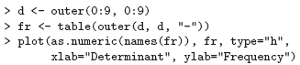
Notice the coercion of the names attribute of the frequency table to numeric in order to recover the range of the determinant values. The “obvious” way of doing this problem with for loops is so inefficient as to be impractical. It is also perhaps surprising that about 1 in 20 such matrices is singular.

Next: Generalized transpose of an array

Summary: Index