The following sections detail many of the commonly-used graphical parameters. The R help documentation for the par() function provides a more concise summary; this is provided as a somewhat more detailed alternative. Graphics parameters will be presented in the following form:

name=value A description of the parameter’s effect. name is the name of the parameter, that is, the argument name to use in calls to par() or a graphics function. value is a typical value you might use when setting the parameter.

Note that axes is not a graphics parameter but an argument to a few plot methods: see xaxt and yaxt.

Graphical elements

R plots are made up of points, lines, text and polygons (filled regions.) Graphical parameters exist which control how these graphical elements are drawn, as follows:

pch="+" Character to be used for plotting points. The default varies with graphics drivers, but it is usually ‘o’. Plotted points tend to appear slightly above or below the appropriate position unless you use "." as the plotting character, which produces centered points.

pch=4 When pch is given as an integer between 0 and 25 inclusive, a specialized plotting symbol is produced. To see what the symbols are, use the command

> legend(locator(1), as.character(0:25), pch = 0:25)

Those from 21 to 25 may appear to duplicate earlier symbols, but can be coloured in different ways: see the help on points and its examples. In addition, pch can be a character or a number in the range 32:255 representing a character in the current font.

lty=2 Line types. Alternative line styles are not supported on all graphics devices (and vary on those that do) but line type 1 is always a solid line, line type 0 is always invisible, and line types 2 and onwards are dotted or dashed lines, or some combination of both.

lwd=2 Line widths. Desired width of lines, in multiples of the “standard” line width. Affects axis lines as well as lines drawn with lines(), etc. Not all devices support this, and some have restrictions on the widths that can be used.

col=2 Colors to be used for points, lines, text, filled regions and images. A number from the current palette (see ?palette) or a named colour.

col.axis

col.lab

col.main

col.sub The color to be used for axis annotation, x and y labels, main and sub-titles, respectively.

font=2 An integer which specifies which font to use for text. If possible, device drivers arrange so that 1 corresponds to plain text, 2 to bold face, 3 to italic, 4 to bold italic and 5 to a symbol font (which include Greek letters).

font.axis

font.lab

font.main

font.sub The font to be used for axis annotation, x and y labels, main and sub-titles, respectively.

adj=-0.1 Justification of text relative to the plotting position. 0 means left justify, 1 means right justify and 0.5 means to center horizontally about the plotting position. The actual value is the proportion of text that appears to the left of the plotting position, so a value of -0.1 leaves a gap of 10% of the text width between the text and the plotting position.

cex=1.5 Character expansion. The value is the desired size of text characters (including plotting characters) relative to the default text size.

Axes and tick marks

Many of R’s high-level plots have axes, and you can construct axes yourself with the low-level axis() graphics function. Axes have three main components: the axis line (line style controlled by the lty graphics parameter), the tick marks (which mark off unit divisions along the axis line) and the tick labels (which mark the units.) These components can be customized with the following graphics parameters.

lab=c(5, 7, 12) The first two numbers are the desired number of tick intervals on the x and y axes respectively. The third number is the desired length of axis labels, in characters (including the decimal point.) Choosing a too-small value for this parameter may result in all tick labels being rounded to the same number!

las=1 Orientation of axis labels. 0 means always parallel to axis, 1 means always horizontal, and 2 means always perpendicular to the axis.

mgp=c(3, 1, 0) Positions of axis components. The first component is the distance from the axis label to the axis position, in text lines. The second component is the distance to the tick labels, and the final component is the distance from the axis position to the axis line (usually zero). Positive numbers measure outside the plot region, negative numbers inside.

tck=0.01 Length of tick marks, as a fraction of the size of the plotting region. When tck is small (less than 0.5) the tick marks on the x and y axes are forced to be the same size. A value of 1 gives grid lines. Negative values give tick marks outside the plotting region. Use tck=0.01 and mgp=c(1,-1.5,0) for internal tick marks.

xaxs="r"

yaxs="i" Axis styles for the x and y axes, respectively. With styles "i" (internal) and "r" (the default) tick marks always fall within the range of the data, however style "r" leaves a small amount of space at the edges. (S has other styles not implemented in R.)

Figure margins

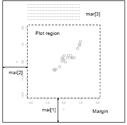
A single plot in R is known as a figure and comprises a plot region surrounded by margins (possibly containing axis labels, titles, etc.) and (usually) bounded by the axes themselves. A typical figure is

Graphics parameters controlling figure layout include:

mai=c(1, 0.5, 0.5, 0) Widths of the bottom, left, top and right margins, respectively, measured in inches.

mar=c(4, 2, 2, 1) Similar to mai, except the measurement unit is text lines.

mar and mai are equivalent in the sense that setting one changes the value of the other. The default values chosen for this parameter are often too large; the right-hand margin is rarely needed, and neither is the top margin if no title is being used. The bottom and left margins must be large enough to accommodate the axis and tick labels. Furthermore, the default is chosen without regard to the size of the device surface: for example, using the postscript() driver with the height=4 argument will result in a plot which is about 50% margin unless mar or mai are set explicitly. When multiple figures are in use (see below) the margins are reduced, however this may not be enough when many figures share the same page.

Multiple figure environment

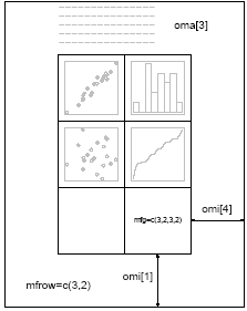
R allows you to create an n by m array of figures on a single page. Each figure has its own margins, and the array of figures is optionally surrounded by an outer margin, as shown in the following figure.

The graphical parameters relating to multiple figures are as follows:

mfcol=c(3, 2)

mfrow=c(2, 4) Set the size of a multiple figure array. The first value is the number of rows; the second is the number of columns. The only difference between these two parameters is that setting mfcol causes figures to be filled by column; mfrow fills by rows. The layout in the Figure could have been created by setting mfrow=c(3,2); the figure shows the page after four plots have been drawn. Setting either of these can reduce the base size of symbols and text (controlled by par("cex") and the pointsize of the device). In a layout with exactly two rows and columns the base size is reduced by a factor of 0.83: if there are three or more of either rows or columns, the reduction factor is 0.66.

mfg=c(2, 2, 3, 2) Position of the current figure in a multiple figure environment. The first two numbers are the row and column of the current figure; the last two are the number of rows and columns in the multiple figure array. Set this parameter to jump between figures in the array. You can even use different values for the last two numbers than the true values for unequally-sized figures on the same page.

fig=c(4, 9, 1, 4)/10 Position of the current figure on the page. Values are the positions of the left, right, bottom and top edges respectively, as a percentage of the page measured from the bottom left corner. The example value would be for a figure in the bottom right of the page. Set this parameter for arbitrary positioning of figures within a page. If you want to add a figure to a current page, use new=TRUE as well (unlike S).

oma=c(2, 0, 3, 0)

omi=c(0, 0, 0.8, 0) Size of outer margins. Like mar and mai, the first measures in text lines and the second in inches, starting with the bottom margin and working clockwise.

Outer margins are particularly useful for page-wise titles, etc. Text can be added to the outer margins with the mtext() function with argument outer=TRUE. There are no outer margins by default, however, so you must create them explicitly using oma or omi. More complicated arrangements of multiple figures can be produced by the split.screen() and layout() functions, as well as by the grid and lattice packages.

Next: Device drivers

Summary: Index