In this section, we analyze the dynamic equilibrium under the general case with fundamental risk, i.e

.. Solving ˙x₂(t) = 0 for the population dynamic in (29)
yields the steady states of the population dynamic. The states x₂ = 0 and x₂ = 1 are always stationary in the dynamic. The long run equilibria of the population dynamic depend critically on the expected return differential in (29). If noise traders have negative average sentiment, i.e. P^¤ < 0, then the expected return differential is negative for all x(t). This means that starting from any nonstationary states the population share of the noise traders will decline to zero in the long run. On the other hand, if noise traders have positive average sentiment in the economy, i.e., P^¤ < 0 , then for some parameter values the expected return differential is positive or all x(t). In this case, starting from any nonstationary states the population share of the noise traders will increase to one in the long run. The third possibility is that for some parameter values the expected return differential is zero. In this case, the dynamic may have at most two interior steady states, denoted by µ_L and µ_h , respectively, as follows,

provided that the expression inside the square roots in (31) and (32) is nonnegative. Following the standard analysis of the dynamic equilibrium in the corresponding evolutionary game (see the Appendix for detail), we obtain the asymptotically stable equilibria for the dynamic in (29) as shown in Theorem 2.2. below:

THEOREM 2.2. In our dynamic playing-the-field contest with fundamental risk, the resulting population dynamic is given in (29). Given the two interior steady states µ_L and µ_h from (31) and (32); respectively; the long run equilibria of the dynamic have four categories.

(I) If noise traders on average have negative sentiment; then rational traders as a group will dominate the economy in the long run.

(II) If noise traders on average have positive sentiment and they always
earns higher expected returns than do the rational traders; regardless of the current population share distribution; then the noise traders as a group will dominate the economy in the long run.

(III) If noise traders on average have positive sentiment and there exists a unique interior steady state; (1 - µ_L , µ_L); then both rational and noise traders will survive in the long run such that their population share distribution approaches the unique interior steady state.

(IV) If noise traders on average have positive sentiment and there exist
two interior steady states; (1 - µ_L , µ_L) and (1 - µ_H , µ_H); then there are two possibilities; depending on the initial population share of the noise traders; x₂(0):

(i) If the noise traders’ initial population share is below ¹H; then both
rational and noise traders will survive such that the population share distribution approaches the lower interior steady state: (1 - µ_L , µ_L).

(ii) If the noise traders’ initial population share is above µ_H ; then the
noise traders as a group will dominate the economy in the long run.

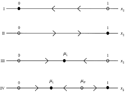
Figure 4 illustrates the evolution of the population share of the noise traders as a group according to Theorem 2.2. The theorem suggests that noise traders vanish in the long run if their average sentiment is bearish, i.e., P^¤ < 0 (category I); otherwise, they always survive under positive sentiment, i.e., P^¤ > 0. Furthermore, noise traders dominate the markets if they always earn higher expected returns than do rational traders, i.e.,

(category II). In category III, starting from any nonstationary states, i.e.,

the population share distribution will converge to the unique asymptotically stable interior equilibrium, (1 - µ_L , µ_L), where both rational and noise traders survive in the long run. Category IV has two interior steady states. Noise traders dominate if their initial population share is greater than the higher interior state µ_H; otherwise,
they survive along with rational traders in the long run as the population
share distribution converges to the unique asymptotically stable interior equilibrium, (1 - µ_L , µ_L). DSSW (1990) obtain similar results regarding the survival of noise traders based on an imitation process where the wealth of trader is held fixed. In fact, DSSW’s long run dynamic with fundamental risk is essentially the same as category IV, while the results for other categories are absent. Therefore, our finding in Theorem 2.2 extends DSSW (1990) by showing that the survival of noise traders is justified even if the wealth accumulation process is endogenously determined.

Theorem 2.2 shows that the categorization depends on the average sentiment parameter, P^¤, and the values of the two interior states, µ_L and µ_H. Hence, we may determine the exogenous parameter space for each category according to the values of these parameters. The parameter space for category I is straightforward to obtain, since it consists of all cases with negative average sentiment, i.e., P^¤ < 0.

FIG. 4. The population dynamic under the playing-the-field contest with fundamental risk.

x2 is the population share of the group of type-2 (i.e., nonrational) traders.

But, obtaining the respective parameter spaces for categories II to IV is difficult. To simplify the matter, define a normalized measure of the average investor sentiment by

, a ratio of the fundamental to noise trader risk by

and aconstant

. Rewrite the expressions of the two interior states µ_L and µ_H in (31) and (32) as follows:

And

Obviously, the two interior states µ_L and µ_H exist only if g > 0. In order to focus on the effects of the average investor sentiment, φ, and the ratio of the fundamental to noise trader risk ψ , fix the constant ς = 3 and the risk-free rate r = 0.05. We can identify the set of the two parameters (φ,ψ) in R²+ that gives rise to each category, respectively, as

and

and

and

and

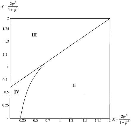
The result is illustrated in Fig. 5 where theψ- φ space

FIG. 5. The categories of the equilibria under positive sentiment.

(II) Nonrational traders dominate rational traders in the long run.
(III) Both rational and nonrational traders survive in the long run.
(IV) Nonrational traders dominate if their wealth share is large enough; otherwise, both types of traders survive in the long run.
¤ Category I corresponds to the case with negative sentiment (i.e., Y < 0) and hence is not shown.

is normalized into X - Y space so that the entire universe R²+ can be shown in the finite space [0,2] x [0,2].

Figure 5 suggests that bullish noise traders dominate the economy only when the fundamental risk is not too small relative to the noise trader risk, i.e.,

and their positive sentiment,

is not too extreme (category II). The intuition is as follows. A relatively large fundamental risk will deter rational traders’ ability and willingness to trade against the mistake of noise traders. A modest positive sentiment allows noise traders to hold more of the risky asset
without causing too much undesirable price impact. As a result, moderately bullish noise traders tend to generate higher expected returns than do the rational traders, particularly when the fundamental risk is large. This implies that in the large economy these modest noise traders as a group will accumulate wealth at a higher speed than will the rational traders. As a result, the noise traders will eventually dominate the market in the long run as their population share increases to one.

On the other hand, if the fundamental risk is small relative to the noise trader risk and the positive sentiment is excessive, then the resulting adverse price impact may be large enough to cancel out the benefit of the positive sentiment. In this case, such bullish noise traders tend to survive but not dominate (category III).

Last, if both the positive sentiment and the fundamental risk are small (category IV), then the noise traders as a group either dominate or survive in the long run, depending on their initial population share relative to the higher interior state, µ_H as described in Theorem 2.2.

Prof. F. Albert Wang

Next: Discussion of Analysis including Empirical Implication

Summary: Index