In this section, we consider noise traders without market power in a playingthe-field contest. Consider a large economy with one riskless asset and N risky assets. The riskless asset is in perfectly elastic supply and pays a fixed dividend r .

The price of the riskless asset is normalized at one and hence the dividend r is also the risk-free rate. The risky asset n (n D 1; 2; : : : ; N) yields an uncertain dividends

at the end of each period t, but its supply is fixed and normalized at one. Assume that the dividends

across time and markets are independently and identically distributed with normal mean r and variance

. While the risky asset’s expected dividend payment r is the same as the riskless rate, the expected total investment returns of the two assets need not be the same. This is so because the risky asset’s price depends on the demand in the market, while the riskless asset’s price is fixed.

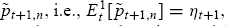
In each asset market n (n = 1, 2........... N), there are many two-period-lived traders. The specific trading mechanism is based on the overlapping generations model of DSSW (1990)3 . Traders of the young generation trade the risky asset n at the market price P_t,n and then liquidate their positions of the risky asset at the price
next period when they become old. As a result, the young traders’ demands for the risky asset n depend on their beliefs about the distribution of the liquidation price next period. Given the identical, normal distributions of fundamental dividends

across markets, the liquidation prices across markets are normally distributed with identical mean N_t+1 and variance

. In each market n, there are two types of traders, depending on their beliefs about the mean, N_t+1 Type-1 (rational) traders accurately perceive the mean of the liquidation prices

while type-2 (noise) traders misperceive the mean N_t+1 by a normal random variable

Note that the superscript i of the expectation operator indicates that the expectation is based on
type-i traders’ beliefs. Following DSSW (1990), let investors’ one-period-ahead expectations about the variance,

, be equal to the variance in the current period, i.e., Ei

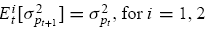. In addition, assume that the misperception variables P_t,n across time and markets are independently and identically distributedwith mean P ^¤ and variance and that they are independent of the fundamental dividents

. Note that the “noise trader risk” is greater if the variance of the misperception variable,

, is greater. All traders have CARA utility with a coefficient
of risk aversion ° . The representative type-i trader in market n chooses a quantity

of the risky asset n to maximize his or her expected utility, given the price P_t,n and the initial capital c₀, as follows:

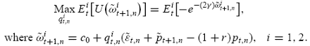
Solving Eq. (20) yields the asset demand for each representative trader as follows:

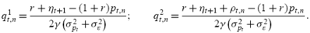
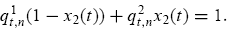
Equation (21) indicates that a bullish noise trader (i.e., P_t,n> 0) holds more of the risky asset than a rational trader does, while a bearish noise trader (i.e., P_t,n< 0) demands less. The market-clearing price is set such that the total demand for asset n equals its total supply (which is normalized to one). Given that the measure of each type of trader in the market is identified with its population share, the market clearing condition is:

Plugging Eq. (21) into (22) and rearranging yields the equilibrium price

as follows:

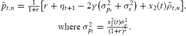
Equation (23) shows that the equilibrium price

in market n depends crucially on the misperception variable

in that market. Given that the misperception variables

across markets are independently and identically distributed, so are the asset prices

across markets. Furthermore, the investment return of the type-i trader in market n, i.e.,

is given by

Since the dividends and the asset prices

are both independently and identically distributed across markets, so are the investment returns

of the type-i traders. The average return of the type-i traders across markets,

, is given by

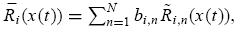where the weight bi;n is the relative size of type-i traders in market n such that the weights across markets sum to one, i.e.

. Given that the individual returns

are independently and identically distributed across markets, the average return converges to the expected investment return of the representative type-i trader, i.e.,

in the large economy. I.e., as

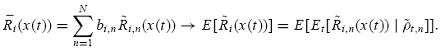
The last equality in Eq. (25) states that the unconditional expected return is the expected value of the conditional expected return, given the misperception variable

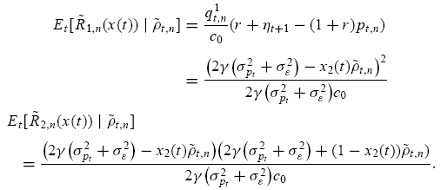
. Using Eqs. (21)–(24), it is straightforward to calculate the conditional expected return for each type of trader as follows:

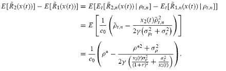
Given (26) and (27), the unconditional expected return differential between the representative type-2 trader and the representative type-1 trader in the economy,
i.e.,

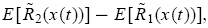is obtained as follows:

Applying Eq. (28) to the general population dynamic in (9) yields the specific population dynamic for the playing-the-field contest (without loss of generality, show the population share for type-2 trader):

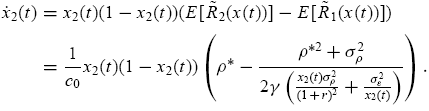
Given the population dynamic in (29), we examine its dynamic equilibrium following the standard analysis in the corresponding evolutionary game. In doing so, we consider first the special case without fundamental risk, i.e.,

, and then the general case with fundamental risk, i.e.,

, respectively.

---

[3] See Kyle (1985), Russell and Thaler (1985), Black (1986), De Long et al. (1989), Campbell and Kyle (1993), Barberis et al. (1998), and Wang (2000) for other noise trading (or investor sentiment) models.

Prof. F. Albert Wang

Next: Dynamic Playing-The-Field Contest without Fundamental Risk

Summary: Index