In our dynamic pairwise contest between rational and nonrational informed traders; the resulting population dynamic is given in (18). The long-run equilibria of the dynamic have four categories; depending on the signs of the return parameters a1 and a2; defined in (18):
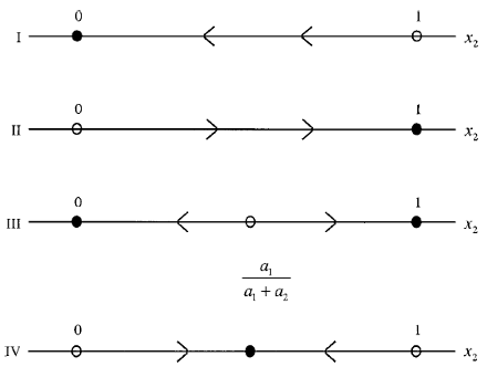
(I) If one always earns a higher expected return by adopting a rational strategy than by adopting a nonrational strategy; regardless of his or her opponent’s type; then rational traders as a group will dominate the economy in the long run.
(II) If one always earns a higher expected return by adopting a nonrational strategy than by adopting a rational strategy; regardless of his or her opponent’s type; then nonrational traders as a group will dominate the economy in the long run.
(III) If one always earns a higher expected return by adopting the same strategy as his or her opponent’s type; then rational (nonrational) traders as a group will dominate the economy in the long run when the initial population share of the nonrational traders; x2(0); is below (above) the threshold level a1=(a1 C a2).
(IV) If one always earns a higher expected return by adopting the opposite strategy of his or her opponent’s type; then both rational and nonrational traders will survive in the long run such that their population share distribution approaches the unique asymptotically stable equilibrium: (a2=(a1 Ca2);a1=(a1 Ca2)).
Figure 1 illustrates the evolution of the population share of the nonrational traders as a group according to Theorem 1. The theorem indicates that nonrational traders dominate in category II, they may dominate in category III if their initial population share is greater than a1=(a1 C a2), and they survive in category IV. But, Theorem 1 does not show whether the nonrational traders in these categories include
both overconfident and underconfident traders, only one kind, or even none if the categories are in fact nonexistent in the model. Note, however, the theorem does show that these results depend on the signs of the two return parameters a1 and a2. It turns out that the signs depend only on two key parameters of the model: the noise-to-signal ratio θ (an inverse measure of the quality of the private signals)

FIG. 1. The population dynamic under the pairwise contest.

x2 is the population share of the group of type-2 (i.e., nonrational) traders.
and the misperception parameter K (an inverse measure of the confidence level of traders.) Recall that an informed trader is overconfident if 0 ≤ K < 1, underconfident if K > 1, and rational if K > 1. We can identify the set of the two parameters θ and K in R2+ that gives rise to each category such that

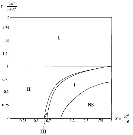
etc. The result is illustrated in Fig. 2 where the θ - K space is normalized into X - Y space so that the entire universe R2+ can be shown equivalently in the finite space [0; 2] x [0; 2]. Several observations about Fig. 2 are in order. First, underconfident traders can never survive in the long run since the entire parameter space for underconfident trading, i.e., K > 1, belongs to category I. In this category, rational traders always
dominate. Second, the survivability of overconfident traders rises with the quality of their private signals and falls with the degree of overconfidence. For example, the figure shows that if the quality of the private signals is sufficiently high, i.e.,

FIG. 2. The categories of the equilibria under the pairwise contest.
(I) Rational traders dominate nonrational traders in the long run.
(II) Nonrational traders dominate rational traders in the long run.
(III) Nonrational traders dominate if their wealth share is large enough; otherwise, rational traders dominate in the long run.
¤ The region NS corresponds to the case where the equilibrium of the one-shot model does not exist.
θ is sufficiently small, overconfident traders, i.e., K < 1, always dominate in category II. One may regard the ex-ante variance of the risky asset value,
 , as the fundamental risk in the economy. Holding forecast error
 constant, then a small
 implies large fundamental risk,
  . In this context, overconfident traders tend to dominate the market when the fundamental risk is large. On the other hand, if the quality of the signals is relatively poor, i.e.,θ is large, then overconfident traders can dominate only if their degree of overconfidence is modest, i.e. K is not too small. This result is similar to Hirshleifer and Luo (2001). This similarity is
remarkable because while fundamental risk is priced in Hirshleifer and Luo with risk-averse traders, the risk is not priced in our model under risk-neutrality. In category III, the outcome depends on the initial population share distribution, x(t), and this category comprises only a small subset of the parameter space R2+ Category IV, where both types of traders survive and coexist, is an empty set. Following Kyle and Wang (1997), region NS in the figure corresponds to the
case where the one-shot model does not have equilibrium. Therefore, for all the parameter space where the equilibrium does exist, given a confidence parameter K, Fig. 2 implies that either rational or overconfident traders will dominate in the long run. However, if nonrational traders’ confidence level, K, changes from time to time due to some exogenous, e.g., psychological, factors, then Fig. 1 suggests that
the competitive advantage of a certain type may shift accordingly over time.
For example, if nonrational traders’ sentiment suddenly shifts from underconfidence to overconfidence, then rational traders tend to lose their competitive advantage to the newly minted overconfident opponents, as the long-run equilibrium now changes from category I to II, etc. The dominance of overconfident traders over their rational opponents depends on two factors. First, overconfidence acts like a commitment device to aggressive trading, which makes their rational opponents less aggressive (Kyle and Wang (1997)). Second, given the private signals, informed traders’ demands are positively correlated with the risky asset’s value. These two factors together imply that, in
comparison to rational traders, overconfident traders tend to buy more of the risky asset when their private signals indicate a positive prospect and sell more when the signals suggest the opposite. As a result, the demand differential between the overconfident traders and their rational opponents tends to be positively correlated with the asset’s value. Such a positive correlation leads to a positive expected
return differential between overconfident and rational traders, i.e.,

, despite the fact that the model assumes risk neutrality. To see
this, using (3) the expected return differential can be expanded as follows:

Although there is no risk premium under risk neutrality, i.e.,  , the expected return differential is positive when the demand differential is positively correlated with the risky asset’s value, i.e.,

As a result, the population share of the overconfident traders increases in the evolutionary process.
Prof. F. Albert Wang
Next: Investor Sentiment in a Playing-the-Field Contest
Summary: Index