GARCH Process
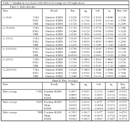
Table 7 repeats the previous results for a simulated GARCH(1,1) model. This model allows for the conditional second moments of the return process to be serially correlated.
Checking the "Buy-Sell" column in Table 7, Panel B, the VMA rule shows that the GARCH model generated an average spread of 0.12 percent, compared with 0.16 percent for the IGBM series. Only 9.13 percent of the simulations generated buy-sell returns as large as those from the IGBM series. The GARCH model generated a positive buy-sell spread that is substantially larger than the spread under the AR(1) process, but this spread is still small when compared with that from the original IGBM series.
In contrast, for both the FMA rule and the TRB rule, the GARCH model generated an average spread higher than those from the IGBM series (2.02 percent and 2.41 percent, compared with 1.67 percent and 2.31 percent for the IGBM series, respectively). The percentage of simulated series that generated a buy-sell returns as large as those from the IGBM series is 56 percent for the FMA rule and 47 percent for the TRB rule. Regarding the simulated buy mean returns, they are lower than the actual mean returns for the VMA and TRB rules, being the associated "p-value" 0.11 and 0.30, respectively.
For the FMA rule, the simulated buy mean returns are higher than the actual mean returns, being the difference highly significant with a "p-value" of 0.66. As for the simulated sell mean returns, they are less negative than the actual sell mean returns for theVMA rule, equal for the FMA rule and more negative for the TRB rule, and the "p-values" of these differences are 0.13, 0.45 and 0.56, respectively. Turning now to volatility, it should be noted that for the IGBM series standard deviations are lower for the buy periods than for the sell periods.
Panel B of Table 7 shows that, for all three trading rules, the average standard deviations for both buys and sells are larger from the GARCH model than those from the IGBM series. For most of the cases, the "p-values" support the significance of these differences. Hence, the GARCH model is substantially overestimating the volatility for both buy and sell periods.
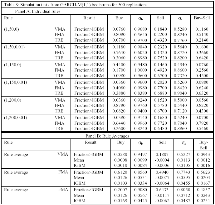
GARCH-M Process
Since a changing conditional mean can potentially explain some of the differences between buy and sell returns, the next simulations examine the GARCHM model. These results are presented in Table 8. In Panel B of Table 8, we see in the "Buy", "Sell" and "Buy-Sell" columns that the results are similar to those from the GARCH. Simulated buy mean returns are similar to those from the GARCH: for the VMA and TRB rules they are lower than the actual mean returns (with associated "p-value" 0.06 and 0.20, respectively), while for the FMA rule, the simulated buy mean returns are higher than the actual mean returns (with a "p-value" of 0.61).
In the case of the simulated sell mean returns, there are some differences with respect to the GARCH results. As can be seen, they are less negative than the actual sell mean returns for the VMA rule, and more negative for the FMA rule and TRB rule, being these differences highly significant as indicated by the "p-values" of 0.18, 0.49 and 0.64, respectively.
Regarding the volatility, as in the GARCH case, for all three trading rules, the average standard deviations for both buys and sells are larger from the GARCH-M model than those from the IGBM series. Nevertheless, we observe some changes in the results when compared to GARCH. For the VMA and the FMA rules, the conditional buy volatilities are lower for the GARCH-M than for the GARCH, while the opposite is true for the dell volatilities. For the TRB rule, the GARCH-M model generated higher buy volatility than the GARCH model, while the conditional sell volatilities are similar for the GARCH-M and for the GARCH.
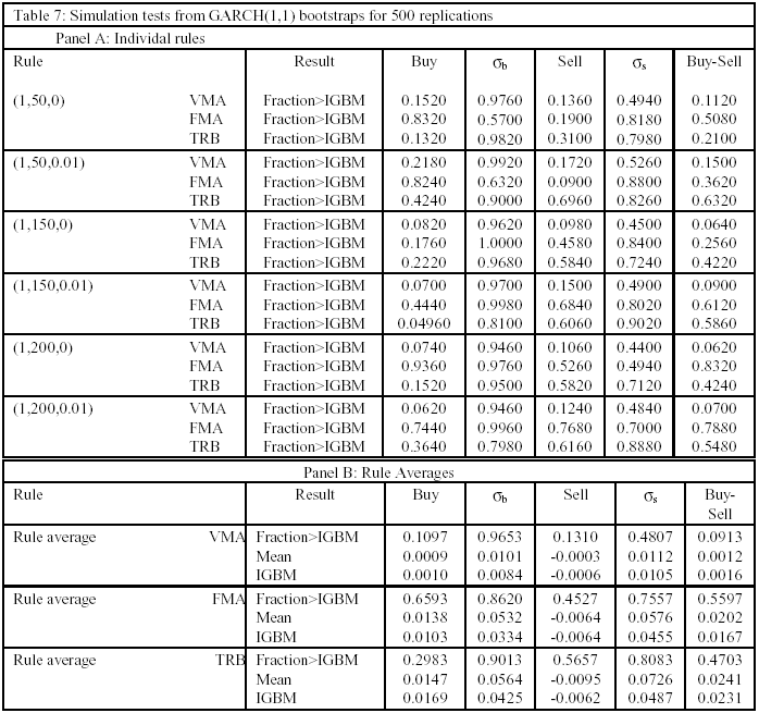
As in Section 3, we have also considered two nonoverlapping subperiods, being 19 October 1987 the breaking point. As before, the results (not present here, but available from the authors upon request) do not suggest significant differences across subperiods.
By F. Fernández, S. Sosvilla and J. Andrada
Next: Concluding remarks
Summary: Index