The results presented in Section 3 indicate that trading rules produce higher returns than the unconditional mean return. However, this conclusion is based on inference from t-statistics that assume independent, stationary and asymptotically normal distributions. As we have seen from Table 1, these assumptions certainly do not characterise the returns from the IGBM series. Following BLL (1992), this problem can be address using bootstrap methods (see Efron and Tibshiarani, 1993), which also facilitate a joint test across different trading rules that are not independent of each other.
The basic idea is to compare the time series properties of a simulated data from a given model with those from the actual data. To that end, we first estimate the postulated model and bootstrap the residuals and the estimated parameters to generate bootstrap samples. Next we compute the trading rule profits for each of the bootstrap samples and compare this bootstrap distribution with the trading rule profits derived in Section 3 from the actual data.
Using information up to and including day t, the trading rules classify each day t as either a buy (bt), a sell (st) or, if a band is used, neutral (nt). If we define the h-day return at t as:
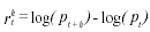
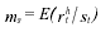
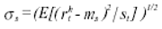
(where p is the level of the index), then the expected h-day return conditional to a buy signal can be defined as
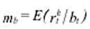
and the expected h-day return conditional to a sell signal can be defined as
The conditional standard deviations may then be defined as
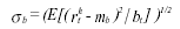
and
These conditional expectations are estimated using appropriate sample means calculated from the IGBM series and compared to empirical-distributions from simulated null models for stock returns. Therefore, the bootstrap methods are use both to assess the profitability of various trading strategies and as a specification tool to obtain some indication of how the null model is failing to reproduce the data. Regarding what model should be used to simulate the comparison series, following BLL (1992) we consider several commonly used models for stock prices: autorregressive process of order one (AR(1)), generalised autorregressive conditional heteroskedasticity model (GARCH) and GARCH in-mean model (GARCH-M).
The first model for simulation is the AR(1)
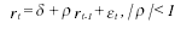
where rt is the return of day t and εt is independent, identically distributed. The parameters (δ and ρ) and the residuals εˆt are estimated from the IGBM series using ordinary least squares (OLS). The residuals are then resampled with replacement and the AR(1)s are generated using the estimated parameters and crumbled residuals.
The second model for simulation is the GARCH(1,1) model
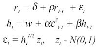
where the residual (εt ) is conditionally normally distributed with zero mean and conditional variance (ht) and its standardized residuals (zt) is i.i.d. N(0,1). This model allows for the conditional second moments of the return process to be serially correlated. This specification incorporates the familiar phenomenon of volatility clustering which is evident in financial market returns: large returns are more likely to be followed by large returns of either sign than by small returns.
The
parameters of the GARCH(1,1) model are estimated from the IGBM series using
maximum likelihood. To adjust for heteroskedasticity, the resampling algorithm is
applied to standardized residuals. Therefore, the heteroskedastic structure captured
in the GARCH(1,1) model is maintained in simulations, and only the i.i.d. standardized residuals ( ) are resampled with replacement.
The last model considered in the simulation is the GARCH(1,1)-M model
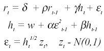
In this specification, the conditional variance is introduced in the mean equation of the model. This is an attractive form in financial applications since it is natural to suppose that the expected return on an asset is proportional to the expected risk of the asset. As in the GARCH(1,1) model, the parameters and standardized residuals are estimated from the IGBM series using maximum likelihood. Once again, the standardized residuals are resampled with replacement and used along with the estimated parameters to generate GARCH-M series.
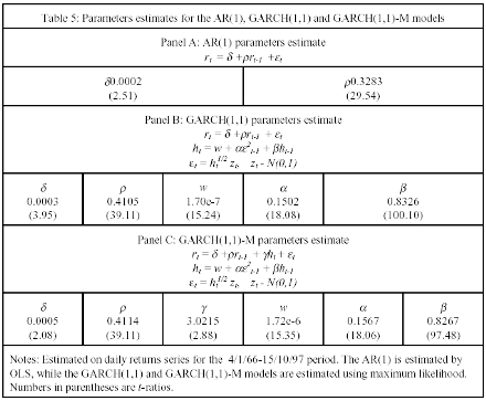
Table 5 presents the estimation results for the AR(1), GARCH(1,1) and GARCH(1,1) models. Panel A shows the results from the estimation of an AR(1) model using OLS. As can be seen, there is a significant first order autocorrelation in the IGBM series. Panel B contains the results from estimation of a GARCH(1,1) model using maximum likelihood. Note that the model estimated also contains an AR(1) term to account for the strong autocorrelation. The estimated parameters α and β indicate that the conditional variance is time varying and strongly persistent.
The variance persistence measure (α + β) is 0.9828. The results are in line with those reported by Olmeda and Pérez (1995) who studied nonlinearity in variance in the IGBM over the 1989-1994 period using a GARCH(1,1) model for the AR(1) residuals of the returns. The • parameter, capturing the first orden autocorrelation in the series, is also significantly positive. Finally, Panel C presents the results for the GARCH(1,1)-M model. As can be seen, the estimate conditional expected return is positively related with the conditional variance (γ=3.02).
By F. Fernández, S. Sosvilla and J. Andrada
Next: AR(1) Process
Summary: Index