Definition Specifically, let s(O) and s(0)' be two initial conditions that are close to each other, i.e. l l s(0) - s(0)'11 < e where 1 1 .11 is any norm and e > 0 is small. Assume for simplicity that the time evolution is discrete. After time N,

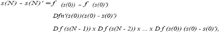
where D f is the Jacobian matrix. Moreover,

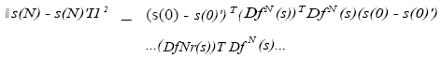
The multiplicative ergodic theorem by Oseledec (1968) states that if we form the so-called Oseledec matrix

then the limit limN-,, OSL(s, N), exists and is independent for p-almost all s in the basin of attraction of the attractor to which the trajectory defined by the dynamical system belongs. The logarithm of the eigenvalues oflimN-,,, OSL(s, N), which is an orthogonal matrix, are denoted by A1 > X> > ... > A and are the global Lyapunov exponents for the dynamical system with respect to the ergodic measure p.

The global Lyapunov exponents give a measure of the average growth or decay of infinitesimal perturbations to a trajectory over a long time.

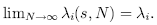
Closely related to the global Lyapunov exponents, hereafter called the Lyapunov exponents, are the local or finite time Lyapunov exponents (Abarbanel et al., 1991). The local Lyapunov exponents

measure how rapidly infinitesimal perturbations to a trajectory at state s grow or shrink in N time steps away from the time of the perturbation.

Often, these exponents vary significantly with the state s on the attractor, especially when N is small, which means that the variation of predictability over the attractor may be large. Of course,

If the largest Lyapunov exponent is positive, i.e.

the system is chaotic and has the aforementioned property of "sensitive dependence on initial conditions".If the system is dissipative then the sum of the Lyapunov exponents is negative, i.e.

and the solution paths remain within a bounded set.

Estimation

Since the seminal paper by Takens (1981), extensive research has been carried out to develop methods for estimating the Lyapunov exponents from an observed scalar time series. The first method was presented by Wolf et al. (1985) and thereafter several methods have been proposed.'

These methods either estimate the largest Lyapunov exponent, the non-negative portion of the Lyapunov exponent spectrum or the entire Lyapunov exponent spectrum.

Most methods are so-called Jacobian methods. Recall that if the delay reconstruction map in eq. (2.5) is an embedding, then the function g in eq. (2.6) is induced on the reconstructed phase space.Since the Lyapunov exponents are computed from Dfⁿ, it is important to estimate Dgⁿ. To simplify the exposition, assume that the reconstruction delay is equal to one and that the reconstruction is predictive in the sense that no data points are taken from the future, i.e. J = 1 and m = 0 in eq. (2.4). This means that the function g may be written as

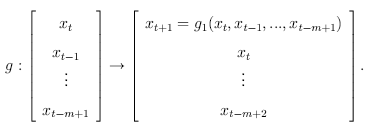
The Jacobian matrix Dg at the reconstructed state xt is

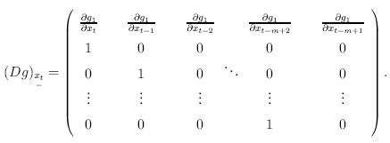
Since

the Lyapunov exponents can be estimated by estimating the Jacobian matrixes along the reconstructed trajectory. For example, Dechert and GenCay (1992) and Gencay and Dechert (1992) consistently estimate the entire Lyapunov exponent spectrum whereas McCaffrey et al. (1992) and Nychka et al. (1992) consistently estimate the largest Lyapunov exponent.
There is, however, a problem with the Jacobian method when estimating the
entire Lyapunov exponent spectrum. This is because the method is applied to the full m-dimensional reconstructed phase space and not just to the n-dimensional manifold which is the image of the delay reconstruction map 4 in eq. (2.5).

As a consequence, m Lyapunov exponents are estimated whereupon n are true Lyapunov exponents and m - n are so-called spurious Lyapunov exponents. Even worse, spurious Lyapunov exponents that are larger than the largest true Lyapunov exponent may be obtained (Dechert and GenCay, 1996). The true Lyapunov exponents can, however, be identified because they change their signs upon time reversal whereas the spurious Lyapunov exponents do not (Parlitz, 1992). It goes without saying that the method does not work when the dynamics fail to be one-to-one.

A simple non-Jacobian method that estimates only the largest Lyapunov exponent was proposed by Rosenstein et al. (1993). This method, which is based on previous work by Eckmann et al. (1986) and Sano and Sawada (1985), is utilized in Papers [i]-[iii] and is as follows: Given a reconstruction of the attractor, i. e. a reconstructed phase space, search for the nearest neighbor of each state on the trajectory:

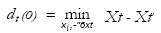
where

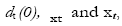
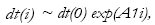
are the distances between the tth state and its nearest neighbor, the reference state and the nearest neighbor, respectively. The tth pair
of nearest neighbors then diverge at a rate approximated by the largest Lyapunov exponent:

(2.8)

where i is the number of steps following the nearest neighbors. Taking the logarithm of both sides of eq. (2.8) gives

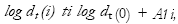
which represents a set of approximately parallel lines each with a slope approximately proportional to A1 . The largest Lyapunov exponent is then estimated using a least-squares fit with a constant to the average line defined by (log dt (i)) where (.) denotes the average over all values of t.

Prof. Mikael Bask

Next: Testing for chaotic dynamics in observed time series

Summary: Index