In the standard asset market approach in exchange rate economics the (log of the) exchange rate e_t is driven by the expected rate of depreciation and a set of contemporaneous fundamentals included in a vector yt. Thus the exchange rate can be written as

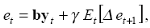(1)

where the vector of elasticities of the contemporaneous variables b and the elasticity of exchange rate expectation γ should be constant over time. For the sake of simplicity, vector y consists only of one variable z with its coefficient denoted by α:

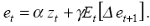(1')

Under the rational expectation hypothesis, equation (1) has the well-known forward-looking solution:

(2)

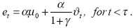
Following Lewis (1989), we assume that fundamental z is stationary, but at time τ a regime shift occurs in its mean. Due to an announcement or an event, agents believe that the regime shift is possible but are not sure whether it in fact occurs at time τ. For example, the central bank may decide to conduct a monetary policy that is suitable to bring down inflation and announces this regime shift at time τ.

Nevertheless, private agents cannot be fully convinced of the announcement, implying that they still assign a positive probability to the prevalence of high inflation monetary policy. Assuming that the market knows the true values of the process before and after the switch, z_t evolves according to

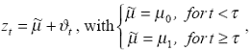(3)

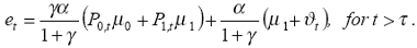
where 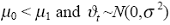. As long as t < τ, the exchange rate can easily be calculated by taking expectations from equation (3) and substituting the result into equation (2):

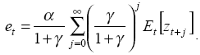
(4)

In the following periods, the market’s uncertainty will be reduced as agents make observations about z over time and discover whether µ₀ or µ₁ is the true mean of the fundamental z. This reduction of uncertainty can be characterized by a learning model, where market participants generate Bayesian forecasts and assign a probability to either process. Defining P_{i, t} as the probability that the process at t > τ is driven byµ _i , the market’s expectation of z_t is

(5)

Probabilities P_{i, t} are updated with every realization of z according to Bayes’ law:

(6)

where is the density function of zt if µ i is the true mean of the process. The odds at time t that the process has switched are 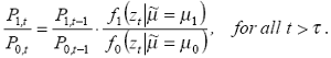(7)

Taking logs and solving the resulting difference equation yields

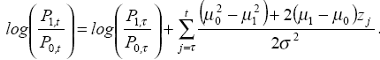(8)

At time τ, when the possibility of a regime shift is perceived, market participants are supposed to believe that one regime is as likely as the other. This implies that log(P_{1, t}/P_{0, t})=0 and

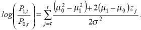(9)

Equation (9) can be solved for the probabilities P_{i, t} using the fact that P_{0, t}=1-P_{1, t}:

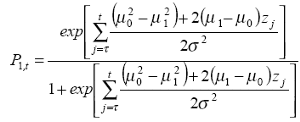(10.1)

and

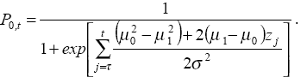(10.2)

Together with eq. (2) and eq. (5), the exchange rate at t > τ is

(11)

The post regime shift equilibrium value of the exchange rate is different to the pre-shock value (eq. (4)) for two reasons. First, according to the second term of eq. (11), contemporaneous realizations of z account for a permanent change in the stochastic process of the exchange rate. We may interpret this source of regime shift as a change in the excess demand of “real bill” export/import traders.

Its magnitude depends on parameter γ and is expected to be small, since balance of payment transactions account for only little trading volume on foreign exchange markets. Second, according to the first term in eq. (11), the exchange rate is driven by agents’ expectations, i.e. the probabilities assigned to either process, which move over time in response to new information regarding the fundamental z. Since in fact there has been a regime shift, probability P_{1, t} converges to one (plim P_{1, t}=1) and

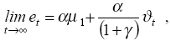(12)

which may be interpreted as the new long-run equilibrium value of the exchange rate. Clearly, based on the ex-post available knowledge of the true stochastic process of z, the forecasting errors are biased over the whole learning process. But note that, conditional on the information available at time t, the expectations of market participants are rational in that they minimize forecast errors.

The path of the exchange rate cannot converge to (12) if fundamental z is currently unobservable. With regard to the topic of this paper, the following cases are worth mentioning. If the regime shift occurs without any announcement, the exchange rate differs from its pre-shock value of (4) solely due to liquidity traders’ activity:

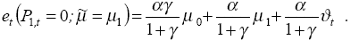(12')

Note that as long as γ > 0, i.e. the extent to which future expected values of the fundamental are discounted to determine the current exchange rate, the level of the exchange rate in (12’) is still different from its long-run equilibrium value. This incomplete adjustment of the current exchange rate is the basis for successful predictions of technical analysis.

As will be discussed in detail in the next section, technical analysis makes use of the information introduced into exchange rate dynamics by liquidity traders’ activity. The sign prediction is confirmed when observations of the fundamental z become available and the standard learning process, as described above, drives the exchange rate towards its new equilibrium value.

However, it must be mentioned that a somewhat persistent exchange rate change may also occur in the prevalence of fads. Assume that noisy information forces market participants to set P_{1, t}>0, but the regime shift does not occur. The mere possibility of the regime shift leads to a change in the exchange rate compared to the pre-shock level:

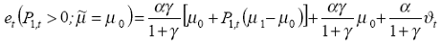(12'')

Obviously, the exchange rate dynamics exhibits a kind of bubble because agents consider a possible path of the fundamental, which never takes place. While technical analysis signals structural breaks in the time series of the exchange rate, it is generally not able to distinguish between the causes of these switches. As a consequence, trading on technical analysis may also bring about bubbles in exchange rates.

Prof. Stefan Reitz

Next: The Derivation of Rational Sign Predictions

Summary: Index