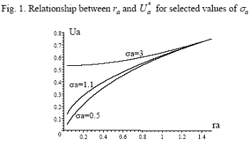
Relationships between the parameters ra, σa, and U*_a .

The contemporaneous relationship between the parameters C*_a, sa, and U*_acan be seen from numerical simulations as depicted in the Figure 1, where ra and U*_a appear in the two axes. The curves are drawn for selected values of σa (0.5, 1.1, and 3 respectively), while the remaining parameters are set thus: α=0.5, A=1.5.

A negative relationship between U*_a and ra may emerge only if, for a diminishing ra, σa at the same time takes very great values. This is the case of individuals of group III.

Proof of Proposition 1.

At the beginning of each period the population of size N consists of 0.5N youths with D^M_yand of 0.5N adults. Adults belong to group I with D^M_a or to groups II and III with D^m_a. Let us call p the share of the population with D^M , i.e.with D^M_y and D^M_a.

A youth will enter group I or group II+III of adults, depending on the share of people with D^M in the sample with whom he has a relationship. Let us call P this share, and n>30 the sample size, equal for each youth. Sampling is with repetition, since a youth can meet many other people, and the size of the population can be regarded as infinity in this case. Sample distribution of P is a binomial one with

Let us call PS the share that makes ry=S in (15), so that a youth enters group I if P>PS, he enters group II or III if P ≤ PS.

The sample is sufficiently great to allow use of the standardised normal distribution zs = (Ps - p)/ σs to calculate the cumulated probability Π, i.e. the region on the right of zS under the curve of the distribution, where P>PS. Let us assume that N is sufficiently great for Π to approximate the share of youths in the population who enter group I. Therefore, in the following period the proportion p includes the new youth and those who entered group I, i.e. It can be stated that PS proves to be ‘too great’ or ‘too small’, i.e. the requirement to enter group I is too tight or too loose, whether it implies or 2 respectively. Therefore, an equilibrium value P*s exists such that P_t=1= P_t=2 and correspondingly S* exists. An equilibrium in the composition of the population can thus be defined. This equilibrium is unstable: if, e.g., P_t=1> P_t=2 , then a greater zs fixes Π_t=1> Π_t=2 , so that P_t=2> P_t=3. Similar arguments apply to P_t=1< P_t=2 and for the subsequent periods.

The growth rate of income per head ( γ) is the sum of the growth rate of productivity per time unit ( γA) and of the change rate of the total time worked (in each period) ( γLT). Whereas γA is assumed to be exogenous and positive, γLT depends on γA. In fact:

If S _t=1 >S*, total working time tends to be performed only by group II, which exhibits σa=1, and by group III, which exhibits σa>1. Therefore, in this case: γ> γA. If S _t=1 < S*, total working time tends to be performed only by group I, which exhibits σa<1. Therefore, in this case: γ< γA.

Proof of Proposition 2.

In the previous proof, the threshold S and the current proportion of the population N with D^M determines the subsequent proportion of group I, which in turn affects the subsequent proportion of N with D^M . Similarly, the threshold s and the current proportion of the population with D^M determines the subsequent proportion of group III. However, the proportion of group III does not affect the subsequent proportion of N with D^M . Therefore, the sizes of groups III and II are determined by both s and S, and thus s determines only the size of group III relative to group II.

By Prof. Maurizio Pugno

Next: References

Summary: Index