A. Pricing analysis for commodity or stock

Denote:

µ----the cost price of commodity, or the average of holding price of all traders in the market to a stock

σ----the standard variance of cost price of commodity.

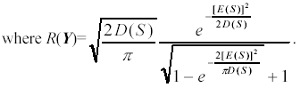
x----the market price variable of a commodity or a stock. thus, R(x) in expression (3) is an average selling profits.

Comparing with Levy distribution,

1) Partial distribution can describe the non-negative characteristic of price of commodities or stocks.

2) Partial distribution can explain that the price of commodity may be zero.

3) The expectation and the variance of partial distribution can be expressed as elementary functions.

4) The average selling profits R(x) in (3) can be estimated.

5) If measure the risk by the variance, we can deduce to that the risk of market price is smaller than the risk of cost price.

Go a step further, if we let Y be a future on underlying S, and S e P( µ, σ²), thus Y e P(E(S), D(S)). We have E(Y)= E(S)+R(Y), D(Y)= D(S)+ E(Y)(E(S)-E(Y)),

Because E(Y)>E(S), then D(Y)<D(S), this means that the risk of future is less than the risk of its underlying.

B. The formulas of American call and put option pricing

We will use the following notation:

t—current time.

S(t)—market price of the underlying at t.

Z—strike price of option on S(t).

T—time of expiration of option.

r—risk-free rate of interest to maturity T.

S(t)e^r(T-t)—forward value of S(t) (Ê(S(T)),the expected value in a risk-neutral world).

Cs—value of call option to buy one share.

Ps—value of put option to sell one share.

1) The price of call option at time t is

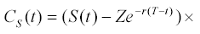
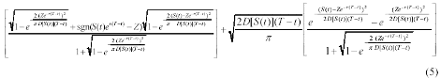
When the call option is brought forward to execute at any time τ e [t,T], the price of underlying stock, S(τ), becomes a constant to the option contract, thus D[S(τ)]=0. According to (5) and theorem 1, the current value of the option is

namely,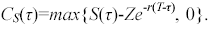

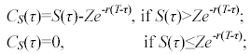
At this time, the intrinsic value of the call option is max {S(τ)-Z,0}, thus

(6)

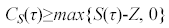
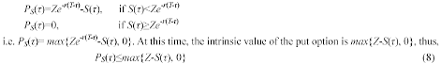
2) The price of put option at time t is

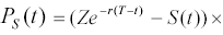
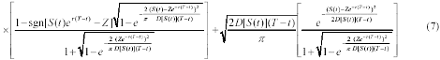
When the put option is brought forward to execute at any time τ e [t, T], the price of underlying, S(τ), becomes a constant to the option contract, thus D[S(τ)]=0. According to (7) and theorem 1, the current value of the option is

3) put-call parity between call and put option prices. According to (5) and (7), we have the following put-call parity:

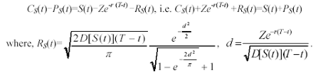
Because we can calculate the partial distribution of S(t) and the D[S(t)] at any time as t goes on, the American put option could be priced.

Prof. Feng Dai

Next: Others Applications

Summary: Index