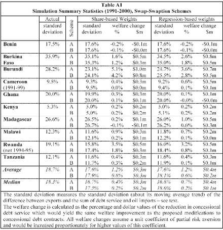
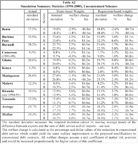
Write the country’s commodity export revenues as X, its oil import expenditures as O and concessional debt service, as modified by the scheme, as R. Then Xt - Ot - Rt is residual forex availability. Without loss of generality, write Rt=St+rt so that r is the change in debt service resulting from the intervention. Write the vector of interventions over the entire simulation as . Let social welfare W have three components:

· the expected utility from consumption C of subsistence goods Z,

· the expected utility obtained from imported consumer goods M, and

· the expected utility of consumption of oil imports.

We suppose that the social welfare function is additively separable both over time and between the first of these components and the remaining two²⁶. Hence, over an H period horizon,

where F is the social discount factor, and

Ignoring, for simplicity, remittances, aid and capital inflows, the balance of payments constraint is Xt=Mt+Ot+Rt . Year t contribution to social welfare becomes

The assumption of additive separability implies that we do not need to consider the second right hand side term in equation (A3) which is independent of rt. For any set of values we may define the reduction d ( ) in debt service that the country would regard as equivalent, in social welfare terms, to the reduction in variability resulting from the choice of non-zero interventions . This reduction is defined implicitly by the equation

Write the expected period t utility level in the absence of intervention (i.e. rt = 0) and with commodity exports, oil imports and debt service all at their moving average levels as

Expanding equation (A4) around the (centred) moving average trend values

we obtain

To a first order approximation, we may assume the marginal utilities are constant.

Further, in order to simplify the resulting expressions, we assume that the curvatures

are constant where is the average level of commodity exports over the period t = 1,…,H²⁷.

Then, by virtue of equation (2), the first term on the right hand side of equation (A5) is zero and the equation may be written as

the reduction (measured as positive) in the year t proportionate variance. If we assume this reduction is independent over time and take the horizon H to be large, the equivalent proportionate reduction in debt is

where

the coefficient of partial risk aversion – see Zeckhauser and Keeler (1970)

and

the scaled ratio of the NPV of debt service to exports. In what follows, we approximate

to avoid making assumptions on discount rates.

 

26 This formulation implies limited substitutability between non-oil imports on the one hand and oil and subsistence goods on the other. That assumption is required to allow a monotonic relationship between free forex and social welfare.

27 This assumption, made for analytical convenience, implies that relative risk aversion declines as commodity export revenues increase. This may be reasonable.

By Prof. Christopher L. Gilbert, Prof. Alexandra Tabova

Next: References

Summary: Index