A market is said efficient if prices reflect all the available information, that is, a speculator cannot make a profit with probability one in the long run. Evidence for a certain degree of inefficiency in financial markets has been recently found (see for example [17]).

Our price dynamics model points out that there exists a contribution in price formation of non random nature and, therefore, it is interesting to check if the associated information is fully absorbed by the market or partially left available for speculators. In this section we set up trading strategies based on our model, which will be applied to financial datasets in the next section: a performance much more successful than the implicit growth of the crude data, given by a buy and hold strategy, will imply a clear evidence of inefficiency.

In order to do this check, let us consider a Kelly-like scheme of repeated investments [18]: Kelly considered a long run of repeated random events, being fixed the probability of the outcome of a single event and the fraction of capital bet at each time. He proved that the capital growth rate is a non random quantity in the limit of infinite events (in this limit the probability of have a growth rate dierent from the typical value goes to zero).

Then he was able to maximize the capital growth rate with respect to the fraction of capital invested, showing a linear relation between the rate itself and the Shannon entropy of the random sequence. In our case, given a capital W(t), lt is the fraction invested at time t in an asset of price S(t), which can be modified at each time. Since the price return r(t) in our model depends only on the dierence α (x(t) − ¯x(t)) = αy(t) and on the parameter σ, the same should be true for lt, i.e. lt = l(αy(t), σ). Then the capital W(t) evolves according to

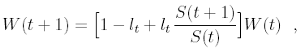
and the associated growth rate is therefore

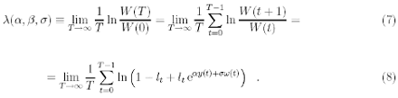
Our goal is to find the optimal l*(αy(t), σ) which gives the maximum growth rate λ*(α, β, σ) for a given set α, β and σ.

Large number theory can be applied to right hand side of (8) since the variables in the sum are weakly correlated in time, in fact, the w(t) are uncorrelated, and the y(t) are related via the moving averages, whose correlations decay exponentially by construction. As a consequence, the fraction of capital invested no longer depends on t, and taking the maximum with respect to l, one has

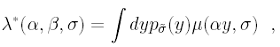
where p˜σ(y) is the steady distribution of variable y, and

where the average h.i is performed over the ω distribution. The maximum in (9) is attained by l = l*(αy, σ), according to the optimal strategy. Let us stress that l must be restricted to 0 ≤ l ≤ 1 if the ω distribution is defined over all reals, to prevent that the logarithm argument in (9) becomes negative. It is easy to show that for symmetric ω distributions the following expressions hold:

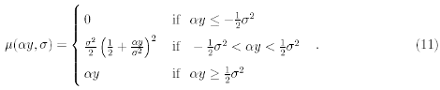
l*(αy, σ) = 1 − l*(−αy, σ) and µ(αy, σ) = αy + µ(−αy, σ). Therefore, when α = 0 the maximum is attained at l*(0, σ) = 1/2, and one has: λ(0, β, σ) = <ln cosh(σω/2)>, which is independent on β.

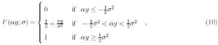
In a more general case, the result strictly depends on ω distribution. Nevertheless, since in real financial data αy and σ are very small (about 1% for daily data, and much lower for intra-day data), it is reasonable to consider a Taylor expansion in αy and σ up to second order. The optimal l*(αy, σ) turns out to be

and, according to this result, one has

In fig. 2 numerical exact results of l*(αy, σ) are plotted for a ω normal distribution and σ = 0.01, compared with approximation (10). In fig. 3 the same comparison is performed for µ(αy, σ), plotting the numerical solution of (9) and the approximation (11). Both graphs reveal the high quality of the approximated solution in a context where variables assume realistic financial values.

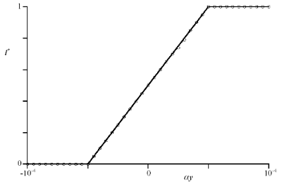
FIG. 2. l*( ay, s ), the value which maximizes the expression (9), as a function of ay for a ? normal distribution and s = 0.01: numerical solution (circles) compared with approximation (10) (continuous line).

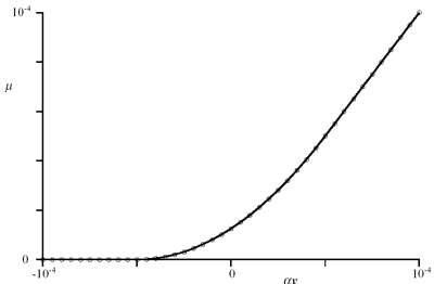
FIG. 3. µ(ay, s) (9) as a function of y for a ! normal distribution and s = 0.01: numerical solution (circles) compared with approximated solution (11) (continuous line).

 

By Prof. R. Baviera, Prof. M. Pasquini, Prof. J. Raboanary and Prof. M. Serva

Next: Forecasting

Summary: Index