The Stochastics establishes a structural relationship between the Close of today and the Maximum and Minimum price of a moving period, measured as the highest High and the lowest Low. Specifying a VAR with the data vector zt = (Ct, Ht max, Lt min) for USDDEM, USDJPY and GBPUSD and testing for cointegration between the three variables should reveal if the Stochastics intuitively exploits Granger causality between these three series.
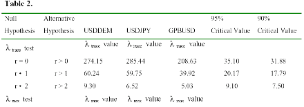
Each VAR included a constant in the cointegration space and 15 lags of each of the variables, which was sufficient to produce random errors18,19. The estimates of λ max and λ trace for the three currencies, reported in Table 2, indicate up to two significant cointegration vectors for USDJPY and GBPUSD and up to three for USDEM. However, based on a graphical inspection of the cointegration relationships, and on an analysis of the companion matrix, we used only the first two vectors for USDDEM.
USDDEM.


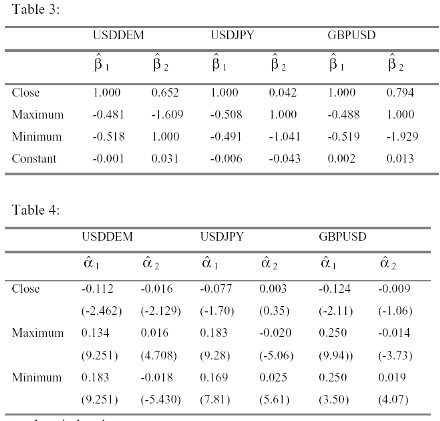
Normalising the first vector on the first element and the second on the third yields the following estimates for β (Table 3) and α (Table 4):

t-values in brackets
$b The results for USDDEM give evidence for two cointegration relationships in the data set comprising Ct , Ht max and Lt min. In the presence of multiple cointegrating vectors, it is now common practice to try to interpret these vectors in an economically and statistically meaningful way. In order to test if these theoretical values are indeed identifying we performed several hypothesis tests.
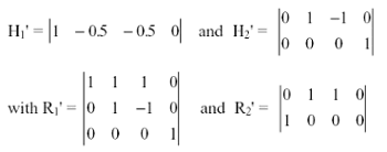
According to Johansen (1992) and Johansen and Juselius (1994) a system is exactly, or just, identified if k = r-1 restrictions are placed on each cointegration vector and the rank condition for generic identification is satisfied. Generic identification requires in the case of two cointegration vectors that the rank condition rank (Ri' Hj) = l 1 for i, j = 1,2 and i ? j is fulfilled. Where Ri is the orthogonal complement of Hi, thus that Ri and Hi are both of full rank and satisfy the conditions Ri 'Hi =0, Ri' βi = 0 and βi= Hi φi . Ri are p*k matrices and Hi are p*s matrices with k + s = p.
If more than k = r - 1 restrictions are placed on each cointegration vector then it is possible to test with a LR test whether these overidentifying restrictions are valid and thus restrict the variation of the parameters. If the overidentifying restrictions satisfy the rank condition and the LR test is passed successfully than each cointegration vector is said to be uniquely identified.
Since the data in this model was constructed imposing the relationship Ct = 0.5(Ht max + Lt min), the estimated coefficients of the normalised first cointegration vector should be close to their theoretical values (1, -0.5, -0.5, 0). We attempt to interpret the second vector as a structural relationship of the form Ht max - Lt min = constant, i.e. a stationary spread between the periodic High and Low prices. In vector form, the second cointegration vector should be of the form (0,1,-1,*).
A test of the first cointegration being equal to (1,-0.5, -0.5,0 ) entails three restrictions on the first cointegration space. A test of the second cointegration being described by (0,1,-1,*) places two restrictions on the second cointegration vector. A joint test of these restrictions is implemented as follows:
 (5)
(5)
The LR test of this model specification has a χ2 distribution with 3 degrees of freedom. For USDDEM the calculated value of χ2 = 4.24 has a p-value of 0.24. Since the rank condition of generic identification is satisfied the statistical model specified by these restrictions is uniquely identifying20. The estimated value of the coefficient of the constant in the second cointegration vector, which is the only freely estimated parameter in the cointegration space, is - 0.041.
This parameter value suggests that the spread between Ht max and Lt min equals 0.041, or 4.1% since log transformed values of the levels were used. The actual average spread between Ht max and Lt min over the period August 1989 - August 1996 was 70 basis points, which translates into 3.8% in log terms. Since the coefficient of the constant has an associated standard error of 0.002, a Wald test of the form

can be used to test the hypothesis that the estimated value equals its empirical counterparts. The Wald statistic, which is asymptotically distributed as χ2 , does not reject this hypothesis since χ2 0.95 = 3.84.
The results of the tests for USDJPY indicate the existence of a similar structural relationship to USDDEM, since the null hypothesis of the first vector being given by (1,-0.5,-0.5,0) and the second being equal to (0,1,-1,*) could not be rejected ( χ2 (2) =1.25, p-value = 0.53).
While the normalised estimates of the cointegration vectors for GBPUSD also seem to suggest a similar structural specification to the cointegration vectors of USDDEM and USDJPY, the LR tests for GBPUSD failed to accept the hypothesis that the first cointegration vector can be identified by (1,-0.5,- 0.5,0). However, the less restrictive test of (1,-0.5, -0.5,*) being part of the first cointegration vector was accepted. The Likelihood Ratio test of this hypothesis is χ2 (1) and the calculated value of χ2 =3.70 has a p-value of 0.05 and is significant at conventional levels.
Since the second cointegration vector of GBPUSD could not be identified as (0,1,-1,*), no evidence for a constant spread between the periodic Highs and Lows could be found for the period. We interpret this as reflective of the sharp depreciation of the Pound against the Dollar after the UK’s decision to leave the ERM in August 1992. The cointegration space for our three exchange rate models is therefore, in the terminology of Johansen and Juselius (1994), not only empirically but also economically identified in the sense that the estimated coefficients can be interpreted from an economical point of view21.
18 The deterministic components of the VAR were defined according to the rank test suggested in Johansen (1992). The rank test facilitates defining the deterministic components of the model together with the rank of the cointegration matrix using the so-called Pantula principle. The rank test suggests the inclusion of a constant in the cointegration space for all three currencies and gave evidence for three cointegration vectors in the case of USDDEM and two for USDJPY and GBPUSD. 19 The model specifications for the three models are presented in the appendix in table 7.
20 Rank Verification of the Rank Condition of Generic Identification of the Long Run Structure:
rank (R1'H2) rank (R2'H1)
21 It is interesting to note that the structural relationships that were identified in the data constructed from the Close and the periodic High and Low series (Ct, Ht max, Lt min ) could not be identified in a data set constructed from daily Close, High and Low series. The Johansen cointegration method revealed also two cointegration vectors for this data set. But even though the cointegration vectors in the data had coefficients quite similar to the two cointegration vectors for USDDEM in the Ct, Ht max, Lt min model, the data for Ct , Ht , Lt failed to accept the hypothesis of vector (1,-0.5, -0.5,*) being part of the cointegration space for all three currencies. This suggests that the relationship C = 0.5(H + L) only holds for periodic High and Low prices of the currencies studied and not for daily High and Low prices and that the cointegration relations between daily data of High, Low and Close seem to follow more complicated dynamics.
Prof. Ronald MacDonald, Prof. Norbert Fiess
Next: Structural Econometric Forecasting Models
Summary: Index