If the RL ascend to a certain degree, the higher foam prospect could be caused. When this kind of higher foam prospect is far from the reasonable APL, the inside force to drive RL to ascend will be exhausted gradually. Also, if RL descend to a certain degree, the lower prospect could be caused. When this kind of lower prospect is far from the reasonable APL, the inside force to drive RL to decline will be exhausted gradually. This exhaustion of force will make the intrinsic trend to move appear reversion. In order to evaluate efficiently the force to drive RL is exhausted or not, and know the terminal of RL going in intrinsic trend, we give out first two assistant functions as follows.

A. Two Assistant Functions

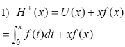(11)

Expression (11) is called the assistant function of ascend behavior of RL.H+(x) means the addition of profiting utility (force of ascending behavior of RL) and the value of RL multiplying the probability of the RL appearing.

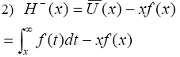(12)

Expression (11) is called the assistant function of descend behavior of RL. H+(x) means the addition of profiting utility (force of descending behavior of RL) and the value of RL multiplying the probability of the RL appearing.

B. The Analytic Indexes

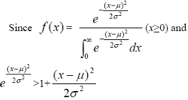
X (RL variable) is assumed to follow Partial distribution, i.e. XεP( µ, σ²).

Definition 4 Let real number l>0 and any x>µ, when H+(x)-U(x) <l, then we call the ascending force of RL is obviously exhausted with l, where l is the fiducial level.

Definition 5 Let real number l>0 and any x, 0<x<µ, when U (x) -H-(x) <l, then we call the descending force of RL is obviously exhausted about l, where l is the fiducial level.

In the Definition 4 and Definition 5, the less the l (obvious level) is, the more the possibility that the inside force to drive RL in intrinsic trend is exhausted is.

the Definition 4 could be explained as: when x (RL) is sufficiently large and the xf(x) (the value of RL multiplying the probability of the RL occurring) is sufficiently small, the high RL is difficult to maintained with long time if probability of the RL appearing is very small. That RL may become the reversing point of ascending trend very much, and at the same time, the ascending force of RL is sufficiently exhausted with l (the significance level); Also, when x (RL) is sufficiently small and the xf(x) is sufficiently small, the low RL is difficult to maintained with long time if probability of the RL appearing is very small. That RL may become the reversing point of descending trend very much, and at the same time, the descending force of RL is sufficiently exhausted with l.

Therefore, according to (11), if want to know whether the ascending force of RL is exhausted or not, we only need to estimate whether x is so large to make xf(x) < l come into existence or not. Or according to (12), we only need to estimate whether x is so small to make xf(x) < l come into existence or not.

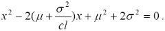
(13)

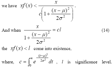
Expression (14) can be written as

According to (4) and (5), we get

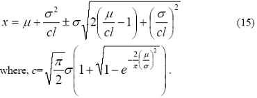
Therefore, on the ascending trend and with the significance level l, the possible highest value of RL reversing is

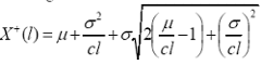(16)

and that, on the descending trend and with the significance level l, the possible lowest value of RL reversing is

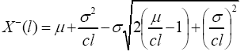(17)

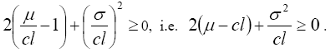
Here we need to see, when |x-µ| is larger, i.e. x away from µ, the left of inequation (13) is obviously larger than the right of inequation (13), for all that, and it will be made clear in the following examples that calculating formula (16) and (17) can't be influenced to apply. By using (16) and (17), we can calculate the equilibrium value of RL ascending or descending.

Denoting:

(18)

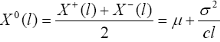
We call X ⁰(l) the equilibrium value of RL, and EV for short.

From (15), we have

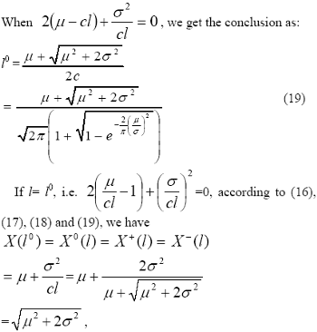
and call 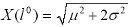the focus value of RL, FV for short. FV reflects basic status of RL in the kernel meanings. So, FV can be used for the judgment that RL is of consistence to proper value or not in some period and on the basic meaning.

C. Determining the Significance Level

If the value of l, the significance level, is too small, it will cause reversing values calculated by (16) and (17) to be too high in ascending trend or too low in descending trend; and If the value of l is too large, it will cause reversing values calculated by (16) and (17) to be too low in ascending trend or too high in descending trend. The two kinds of cases are all difficult to use for practice. Therefore, we can usually determine the value field of l by using of following inequation (19).

(20)

where, l⁰ is determined by expression (19). In usually, the value of l could be larger when the σ, standard variance of APL, is smaller; and the value of l should be smaller when the σ is larger.

D. The examples

In all of the following examples, the parameters, such as µ and σ, is estimated by the method in [14],[15], and the estimated parameters all pass the statistic test of significance.

1) DJX (1/100DJ INDU). We take the close points of DJX as sample data. Time: Jun. 19, 2002—Dec. 24, 2002. The estimated values of parameters in partial distribution P ( µ,σ²) are as follows:

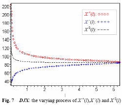
The estimated value of µ is ˆµ =84.84577713, and the estimated value of σ is ˆσ² =28.65615031. So the DJX index follows the partial distribution P(84.84577713, 28.65615031) in the period of time mentioned above. By using of (19), we calculate the l⁰=6.335679489, and the FL, focus level of RL, is: X (l⁰) =85.01448140. When 0<l≤l⁰, the varying process of X⁺ (l), X^- (l) and are X⁰ (l) shown in Fig.7.

Let and by (16) and (17), we get X ⁺ (l)= 99.35843320, X^-(l)=73.02971640. And in the period of time: Jun. 19, 2002 -Dec. 24, 2002, the actual maximum value of DJX is Xmax=95.62, and the minimum value of DJX is Xmin=72.86.

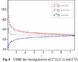
2) CSMI(China Shengzhen stock market index). We take the close points of CSMI as sample data. Time: Apr. 2, 2002—Oct. 8, 2002. The estimated values of parameters in partial distribution P ( µ,σ²) are as follows:

The estimated value of µ is ˆµ =478.0363182, and the estimated value of σ is ˆσ² = 650.3925613. So the CSMI index follows the partial distribution P(478.0363182, 650.3925613) in the period of time mentioned above. By using of (19), we calculate the l⁰=7.488587154, and the FV, focus value of RL, is: X (l⁰) =478.7161101. When 0<l≤l⁰, the varying process of X⁺ (l), X^- (l) and are X⁰ (l) shown in Fig.8.

Let and by (16) and (17), we get X ⁺ (l)= 533.2262202, X^-(l)=430.9981354. And in the period of time: Apr. 2, 2002—Oct. 8, 2002, the actual maximum value of CSMI is Xmax= 512.38, and the minimum value of CSMI is Xmin=429.47.

3) ZYIC(Zongyi Incorporated Company). We take the close points of ZYIC as sample data. Time: Jan. 23, 2002—Aug. 8, 2002. The estimated values of parameters in partial distribution P ( µ,σ²) are as follows:

The estimated value of µ is ˆµ =12.84800010, and the estimated value of σ is ˆσ² = 1.915181026. So the ZYIC index follows the partial distribution P(12.84800010, 1.915181026) in the period of time mentioned above. By using of (19), we calculate the l⁰=3.725104101, and the FV, focus value of RL, is: X (l⁰) =12.92231742.

When 0<l≤l⁰, the varying process of X⁺ (l), X^- (l) and are X⁰ (l) shown in Fig.9.

Let and by (16) and (17), we get X ⁺ (l)= 16.25168021, X^-(l)=10.39286193. And in the period of time: Jan. 23, 2002— Aug. 8, 2002, the actual maximum value of ZYIC is Xmax= 14.68, and the minimum value of ZYIC is Xmin=10.41.

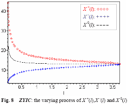
In the example 2) and example 3), the actual maximum values of CSMI and ZYIC (533.2262202 and 16.25168021) are all separately lower than the theoretic maximum values. The reason is that China stock market is in the slumping trend at this time.

Prof. Feng Dai, Prof. Song-tao Wu, Prof. Ya-jun Zhuang

Next: The Calculating Formula for the optimal value for RL

Summary: Index