If we want to price a financial instrument that follows the next SDEs:

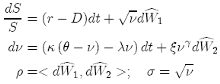(44)

we can use a Monte Carlo scheme to calculate risk-neutral expectations and, using its payoff "Ψ”, we can price it.

VA(S, T) = Ψ(S, K, T )

The accuracy of the option price will mainly depend on:

• What kind of approximation you use to simulate the SDEs.

• The number of Monte Carlo simulations.

• The size of the time step dt. However, if we know the explicit solution of {44}:

VH (S, T) = VH (S0, σ0, T, K, r, D, κ, θ, ξ, γ, ρ, λ)

we can compare the different approximations for various dt and the number of simulations in the Monte Carlo scheme. Then, we define the error by:

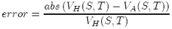(45)

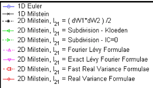
In summary, we want to compare the option price error {45} using Euler and Milstein schemes. To accomplish this, we have to use the Euler and Milstein (1D & 2D) approximations for {44} given in equations {16}, {17}, and {19} respectively and the exact solution formulae for Heston volatility {51}. To simulate the double integral in the 2D Milstein scheme, we use all the approximations defined in section 5 (pages 12-21).

We begin by using a simple example:

Price parameters = (S0 = 700, σ0 = 0.20, K = 700, r = 0.05, D = 0.02) Heston parameters = (κ = 3, θ = 0.07, ξ = 0.35, γ = 0.5, ρ = 0.5, λ = 0) Simply vanilla option, Double integral = (NK = 500 - subdivision methods)

If we simulate all approximations using 5000 simulations in Monte Carlo for various dt, we obtain the following results:

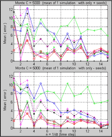
Figure 2.7.- Comparison of all approximation methods using only one set with 5000 Monte Carlo simulations (M.C.).

We can see in figure 2.7 that we obtain different results in both plots. This is because we have used different sets of random numbers. Therefore, it is very difficult to make a good comparison between all of them. However, if we simulate all the processes twenty five times using independent sets of random numbers and then plot the mean of the results, we see (figure 2.8) that the results begin to converge to one value.

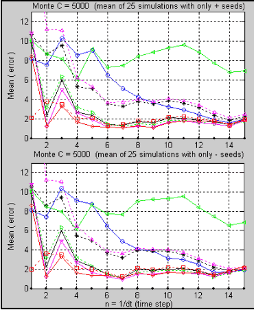
Figure 2.8.- Comparison of all approximation methods using the mean of 25 independent sets with 5000 Monte Carlo simulations (M.C.).

Furthermore, if we simulate 200 times (figure 2.9), we find, surprisingly, that all approximations converge to a single value, and both plots have a very similar shape even though they are simulated with a different set of random numbers. Therefore, we can say that we have calculated the right mean error {45} or right probability for each approximation. Now we can compare them.

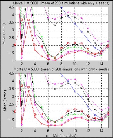
Figure 2.9.- Comparison of all approximation methods using the mean of 200 independent sets with 5000 Monte Carlo simulations (M.C.).

Another important point to notice is that, when dt gets smaller, all approximations must begin to give the same results and, clearly, this is what happens. Because the subdivision methods take a lot of computation time to simulate each time step, we set NK = 1 in figures 2.9 − 2.12. By doing this, the approximation Subdivision IC = 0 (the green line) uses the double integral equal to zero. We can see that it gives approximately the same results as the 1D Milstein scheme and, at some points, it is better. To determine how much all of the approximations vary in their results, we plot the variance of the results shown in figure 2.9 (figure 2.10).

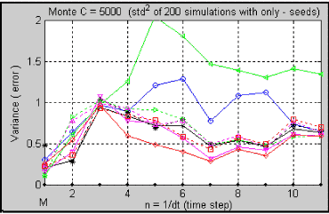
Figure 2.10.- Variance of 200 independent sets with 5000 M.C.

Using the same procedure, the following plots are the results for 625, 1111 and 2500 Monte Carlo simulations.

Figure 2.11.- Mean of 450 independent sets with 2500 M.C.

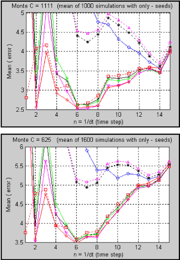
Figure 2.12.- Mean of 1000 and 1600 independent sets with 1111 and 625 M.C.

Because our research focus is to measure accuracy, we have constructed in [13] a large plot matrix that shows all combinations using 100, 400, 625, 1111, 2500, 5000, 6666, 10000, 20000, 50000, 100000 Monte Carlo simulations vs. 1, 10, 25, 50, 75, 100, 200, 450 sets of independent subroutines. The purpose is to explore both the accuracy of all approximations and the time computation when the right mean error {45} or right probability for each scheme is calculated.

Prof. Klaus Schmitz

Next: Conclusions and Observations

Summary: Index